SmoothGrad was introduced by D. Smilkov et al. (2017) and is an extension
to the classical Vanilla Gradient method. It takes the mean of the
gradients for n perturbations of each data point, i.e., with
\(\epsilon \sim N(0,\sigma)\)
$$1/n \sum_n d f(x+ \epsilon)_j / d x_j.$$
Analogous to the Gradient\(\times\)Input method, you can also use the argument
times_input to multiply the gradients by the inputs before taking the
average (SmoothGrad\(\times\)Input).
The R6 class can also be initialized using the run_smoothgrad function
as a helper function so that no prior knowledge of R6 classes is required.
Direct torch alternative
For torch models, a lightweight alternative is available via
torch_smoothgrad that uses native torch autograd directly without
requiring the Converter step. Raw tensor results can be wrapped
into the standard innsight format using as_innsight_result.
References
D. Smilkov et al. (2017) SmoothGrad: removing noise by adding noise. CoRR, abs/1706.03825
See also
Other methods:
ConnectionWeights,
DeepLift,
DeepSHAP,
ExpectedGradient,
Gradient,
IntegratedGradient,
LIME,
LRP,
SHAP
Super classes
innsight::InterpretingMethod -> innsight::GradientBased -> SmoothGrad
Public fields
n(
integer(1))
Number of perturbations of the input data (default: \(50\)).noise_level(
numeric(1))
The standard deviation of the Gaussian perturbation, i.e., \(\sigma = (max(x) - min(x)) *\)noise_level.
Methods
Method new()
Create a new instance of the SmoothGrad R6 class. When initialized,
the method SmoothGrad or SmoothGrad\(\times\)Input is applied to
the given data and the results are stored in the field result.
Usage
SmoothGrad$new(
  converter,
  data,
  channels_first = TRUE,
  output_idx = NULL,
  output_label = NULL,
  ignore_last_act = TRUE,
  times_input = FALSE,
  n = 50,
  noise_level = 0.1,
  verbose = interactive(),
  dtype = "float"
)
Arguments
converter(
Converter)
An instance of theConverterclass that includes the torch-converted model and some other model-specific attributes. SeeConverterfor details.data(
array,data.frame,torch_tensororlist)
The data to which the method is to be applied. These must have the same format as the input data of the passed model to the converter object. This means eitheran
array,data.frame,torch_tensoror array-like format of size (batch_size, dim_in), if e.g., the model has only one input layer, ora
listwith the corresponding input data (according to the upper point) for each of the input layers.
channels_first(
logical(1))
The channel position of the given data (argumentdata). IfTRUE, the channel axis is placed at the second position between the batch size and the rest of the input axes, e.g.,c(10,3,32,32)for a batch of ten images with three channels and a height and width of 32 pixels. Otherwise (FALSE), the channel axis is at the last position, i.e.,c(10,32,32,3). If the data has no channel axis, use the default valueTRUE.output_idx(
integer,listorNULL)
These indices specify the output nodes for which the method is to be applied. In order to allow models with multiple output layers, there are the following possibilities to select the indices of the output nodes in the individual output layers:An
integervector of indices: If the model has only one output layer, the values correspond to the indices of the output nodes, e.g.,c(1,3,4)for the first, third and fourth output node. If there are multiple output layers, the indices of the output nodes from the first output layer are considered.A
listofintegervectors of indices: If the method is to be applied to output nodes from different layers, a list can be passed that specifies the desired indices of the output nodes for each output layer. Unwanted output layers have the entryNULLinstead of a vector of indices, e.g.,list(NULL, c(1,3))for the first and third output node in the second output layer.NULL(default): The method is applied to all output nodes in the first output layer but is limited to the first ten as the calculations become more computationally expensive for more output nodes.
output_label(
character,factor,listorNULL)
These values specify the output nodes for which the method is to be applied. Only values that were previously passed with the argumentoutput_namesin theconvertercan be used. In order to allow models with multiple output layers, there are the following possibilities to select the names of the output nodes in the individual output layers:A
charactervector orfactorof labels: If the model has only one output layer, the values correspond to the labels of the output nodes named in the passedConverterobject, e.g.,c("a", "c", "d")for the first, third and fourth output node if the output names arec("a", "b", "c", "d"). If there are multiple output layers, the names of the output nodes from the first output layer are considered.A
listofcharactor/factorvectors of labels: If the method is to be applied to output nodes from different layers, a list can be passed that specifies the desired labels of the output nodes for each output layer. Unwanted output layers have the entryNULLinstead of a vector of labels, e.g.,list(NULL, c("a", "c"))for the first and third output node in the second output layer.NULL(default): The method is applied to all output nodes in the first output layer but is limited to the first ten as the calculations become more computationally expensive for more output nodes.
ignore_last_act(
logical(1))
Set this logical value to include the last activation functions for each output layer, or not (default:TRUE). In practice, the last activation (especially for softmax activation) is often omitted.times_input(
logical(1)
Multiplies the gradients with the input features. This method is called SmoothGrad\(\times\)Input.n(
integer(1))
Number of perturbations of the input data (default: \(50\)).noise_level(
numeric(1))
Determines the standard deviation of the Gaussian perturbation, i.e., \(\sigma = (max(x) - min(x)) *\)noise_level.verbose(
logical(1))
This logical argument determines whether a progress bar is displayed for the calculation of the method or not. The default value is the output of the primitive R functioninteractive().dtype(
character(1))
The data type for the calculations. Use either'float'fortorch_floator'double'fortorch_double.
Examples
# ------------------------- Example 1: Torch -------------------------------
library(torch)
# Create nn_sequential model and data
model <- nn_sequential(
nn_linear(5, 10),
nn_relu(),
nn_linear(10, 2),
nn_sigmoid()
)
data <- torch_randn(25, 5)
# Create Converter
converter <- convert(model, input_dim = c(5))
# Calculate the smoothed Gradients
smoothgrad <- SmoothGrad$new(converter, data)
# You can also use the helper function `run_smoothgrad` for initializing
# an R6 SmoothGrad object
smoothgrad <- run_smoothgrad(converter, data)
# Print the result as a data.frame for first 5 rows
head(get_result(smoothgrad, "data.frame"), 5)
#> data model_input model_output feature output_node value pred
#> 1 data_1 Input_1 Output_1 X1 Y1 0.008434887 0.4277466
#> 2 data_2 Input_1 Output_1 X1 Y1 0.047988225 0.3907402
#> 3 data_3 Input_1 Output_1 X1 Y1 0.101554558 0.5268267
#> 4 data_4 Input_1 Output_1 X1 Y1 0.117510282 0.5148517
#> 5 data_5 Input_1 Output_1 X1 Y1 0.092038557 0.4672001
#> decomp_sum decomp_goal input_dimension
#> 1 0.01117601 -0.29105106 1
#> 2 0.06522002 -0.44420189 1
#> 3 0.11555072 0.10740989 1
#> 4 0.21758393 0.05942425 1
#> 5 0.13233278 -0.13138849 1
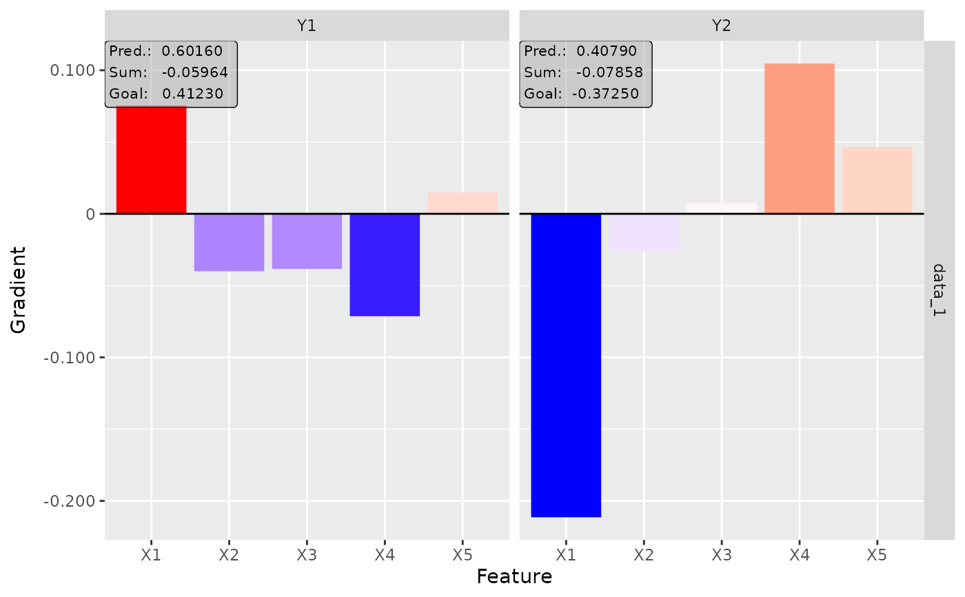
# Plot the result for both classes
plot(smoothgrad, output_idx = 1:2)
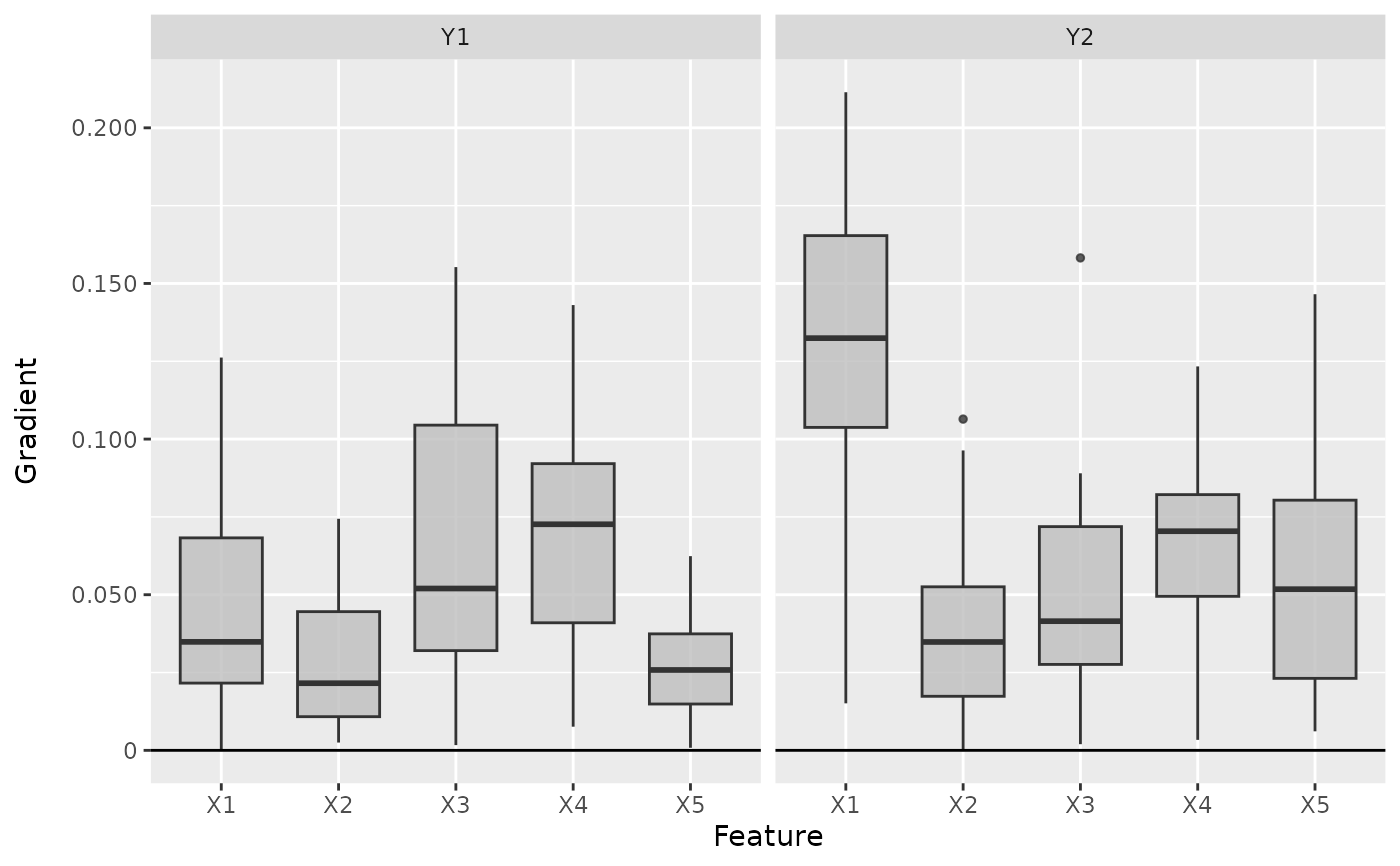
 # Plot the boxplot of all datapoints
boxplot(smoothgrad, output_idx = 1:2)
# Plot the boxplot of all datapoints
boxplot(smoothgrad, output_idx = 1:2)
 # ------------------------- Example 2: Neuralnet ---------------------------
if (require("neuralnet")) {
library(neuralnet)
data(iris)
# Train a neural network
nn <- neuralnet(Species ~ ., iris,
linear.output = FALSE,
hidden = c(10, 5),
act.fct = "logistic",
rep = 1
)
# Convert the trained model
converter <- convert(nn)
# Calculate the smoothed gradients
smoothgrad <- run_smoothgrad(converter, iris[, -5], times_input = FALSE)
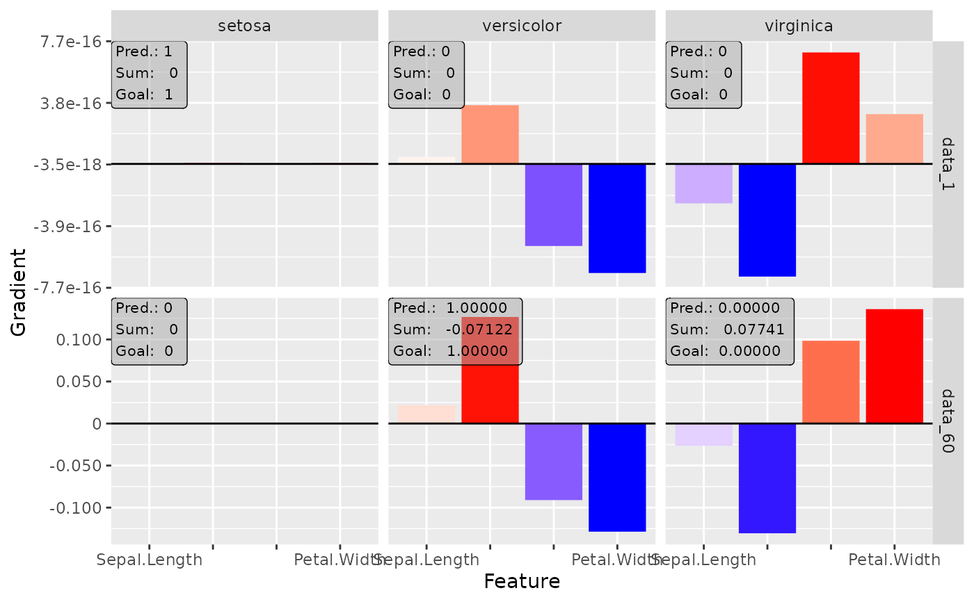
# Plot the result for the first and 60th data point and all classes
plot(smoothgrad, data_idx = c(1, 60), output_idx = 1:3)
# Calculate SmoothGrad x Input and do not ignore the last activation
smoothgrad <- run_smoothgrad(converter, iris[, -5], ignore_last_act = FALSE)
# Plot the result again
plot(smoothgrad, data_idx = c(1, 60), output_idx = 1:3)
}
# ------------------------- Example 2: Neuralnet ---------------------------
if (require("neuralnet")) {
library(neuralnet)
data(iris)
# Train a neural network
nn <- neuralnet(Species ~ ., iris,
linear.output = FALSE,
hidden = c(10, 5),
act.fct = "logistic",
rep = 1
)
# Convert the trained model
converter <- convert(nn)
# Calculate the smoothed gradients
smoothgrad <- run_smoothgrad(converter, iris[, -5], times_input = FALSE)
# Plot the result for the first and 60th data point and all classes
plot(smoothgrad, data_idx = c(1, 60), output_idx = 1:3)
# Calculate SmoothGrad x Input and do not ignore the last activation
smoothgrad <- run_smoothgrad(converter, iris[, -5], ignore_last_act = FALSE)
# Plot the result again
plot(smoothgrad, data_idx = c(1, 60), output_idx = 1:3)
}
 # ------------------------- Example 3: Keras -------------------------------
if (require("keras") & keras::is_keras_available()) {
library(keras)
# Make sure keras is installed properly
is_keras_available()
data <- array(rnorm(64 * 60 * 3), dim = c(64, 60, 3))
model <- keras_model_sequential()
model %>%
layer_conv_1d(
input_shape = c(60, 3), kernel_size = 8, filters = 8,
activation = "softplus", padding = "valid") %>%
layer_conv_1d(
kernel_size = 8, filters = 4, activation = "tanh",
padding = "same") %>%
layer_conv_1d(
kernel_size = 4, filters = 2, activation = "relu",
padding = "valid") %>%
layer_flatten() %>%
layer_dense(units = 64, activation = "relu") %>%
layer_dense(units = 16, activation = "relu") %>%
layer_dense(units = 3, activation = "softmax")
# Convert the model
converter <- convert(model)
# Apply the SmoothGrad method
smoothgrad <- run_smoothgrad(converter, data, channels_first = FALSE)
# Plot the result for the first datapoint and all classes
plot(smoothgrad, output_idx = 1:3)
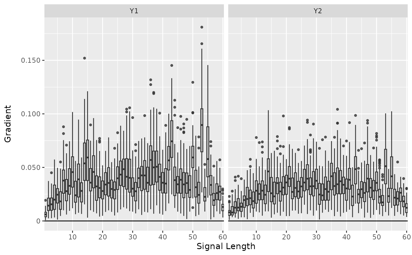
# Plot the result as boxplots for first two classes
boxplot(smoothgrad, output_idx = 1:2)
}
# ------------------------- Example 3: Keras -------------------------------
if (require("keras") & keras::is_keras_available()) {
library(keras)
# Make sure keras is installed properly
is_keras_available()
data <- array(rnorm(64 * 60 * 3), dim = c(64, 60, 3))
model <- keras_model_sequential()
model %>%
layer_conv_1d(
input_shape = c(60, 3), kernel_size = 8, filters = 8,
activation = "softplus", padding = "valid") %>%
layer_conv_1d(
kernel_size = 8, filters = 4, activation = "tanh",
padding = "same") %>%
layer_conv_1d(
kernel_size = 4, filters = 2, activation = "relu",
padding = "valid") %>%
layer_flatten() %>%
layer_dense(units = 64, activation = "relu") %>%
layer_dense(units = 16, activation = "relu") %>%
layer_dense(units = 3, activation = "softmax")
# Convert the model
converter <- convert(model)
# Apply the SmoothGrad method
smoothgrad <- run_smoothgrad(converter, data, channels_first = FALSE)
# Plot the result for the first datapoint and all classes
plot(smoothgrad, output_idx = 1:3)
# Plot the result as boxplots for first two classes
boxplot(smoothgrad, output_idx = 1:2)
}
 #------------------------- Plotly plots ------------------------------------
if (require("plotly")) {
# You can also create an interactive plot with plotly.
# This is a suggested package, so make sure that it is installed
library(plotly)
# Result as boxplots
boxplot(smoothgrad, as_plotly = TRUE)
# Result of the second data point
plot(smoothgrad, data_idx = 2, as_plotly = TRUE)
}
#------------------------- Plotly plots ------------------------------------
if (require("plotly")) {
# You can also create an interactive plot with plotly.
# This is a suggested package, so make sure that it is installed
library(plotly)
# Result as boxplots
boxplot(smoothgrad, as_plotly = TRUE)
# Result of the second data point
plot(smoothgrad, data_idx = 2, as_plotly = TRUE)
}