The DeepSHAP method extends the DeepLift technique by not only
considering a single reference value but by calculating the average
from several, ideally representative reference values at each layer. The
obtained feature-wise results are approximate Shapley values for the
chosen output, where the conditional expectation is computed using these
different reference values, i.e., the DeepSHAP method decompose the
difference from the prediction and the mean prediction \(f(x) - E[f(\tilde{x})]\)
in feature-wise effects. The reference values can be passed by the argument
data_ref.
The R6 class can also be initialized using the run_deepshap function
as a helper function so that no prior knowledge of R6 classes is required.
References
S. Lundberg & S. Lee (2017) A unified approach to interpreting model predictions. NIPS 2017, p. 4768–4777
See also
Other methods:
ConnectionWeights,
DeepLift,
ExpectedGradient,
Gradient,
IntegratedGradient,
LIME,
LRP,
SHAP,
SmoothGrad
Super class
innsight::InterpretingMethod -> DeepSHAP
Public fields
rule_name(
character(1))
Name of the applied rule to calculate the contributions. Either'rescale'or'reveal_cancel'.data_ref(
list)
The passed reference dataset for estimating the conditional expectation as alistoftorch_tensorsin the selected data format (fielddtype) matching the corresponding shapes of the individual input layers. Besides, the channel axis is moved to the second position after the batch size because internally only the format channels first is used.
Methods
Method new()
Create a new instance of the DeepSHAP R6 class. When initialized,
the method DeepSHAP is applied to the given data and the results are
stored in the field result.
Usage
DeepSHAP$new(
  converter,
  data,
  channels_first = TRUE,
  output_idx = NULL,
  output_label = NULL,
  ignore_last_act = TRUE,
  rule_name = "rescale",
  data_ref = NULL,
  limit_ref = 100,
  winner_takes_all = TRUE,
  verbose = interactive(),
  dtype = "float"
)
Arguments
converter(
Converter)
An instance of theConverterclass that includes the torch-converted model and some other model-specific attributes. SeeConverterfor details.data(
array,data.frame,torch_tensororlist)
The data to which the method is to be applied. These must have the same format as the input data of the passed model to the converter object. This means eitheran
array,data.frame,torch_tensoror array-like format of size (batch_size, dim_in), if e.g., the model has only one input layer, ora
listwith the corresponding input data (according to the upper point) for each of the input layers.
channels_first(
logical(1))
The channel position of the given data (argumentdata). IfTRUE, the channel axis is placed at the second position between the batch size and the rest of the input axes, e.g.,c(10,3,32,32)for a batch of ten images with three channels and a height and width of 32 pixels. Otherwise (FALSE), the channel axis is at the last position, i.e.,c(10,32,32,3). If the data has no channel axis, use the default valueTRUE.output_idx(
integer,listorNULL)
These indices specify the output nodes for which the method is to be applied. In order to allow models with multiple output layers, there are the following possibilities to select the indices of the output nodes in the individual output layers:An
integervector of indices: If the model has only one output layer, the values correspond to the indices of the output nodes, e.g.,c(1,3,4)for the first, third and fourth output node. If there are multiple output layers, the indices of the output nodes from the first output layer are considered.A
listofintegervectors of indices: If the method is to be applied to output nodes from different layers, a list can be passed that specifies the desired indices of the output nodes for each output layer. Unwanted output layers have the entryNULLinstead of a vector of indices, e.g.,list(NULL, c(1,3))for the first and third output node in the second output layer.NULL(default): The method is applied to all output nodes in the first output layer but is limited to the first ten as the calculations become more computationally expensive for more output nodes.
output_label(
character,factor,listorNULL)
These values specify the output nodes for which the method is to be applied. Only values that were previously passed with the argumentoutput_namesin theconvertercan be used. In order to allow models with multiple output layers, there are the following possibilities to select the names of the output nodes in the individual output layers:A
charactervector orfactorof labels: If the model has only one output layer, the values correspond to the labels of the output nodes named in the passedConverterobject, e.g.,c("a", "c", "d")for the first, third and fourth output node if the output names arec("a", "b", "c", "d"). If there are multiple output layers, the names of the output nodes from the first output layer are considered.A
listofcharactor/factorvectors of labels: If the method is to be applied to output nodes from different layers, a list can be passed that specifies the desired labels of the output nodes for each output layer. Unwanted output layers have the entryNULLinstead of a vector of labels, e.g.,list(NULL, c("a", "c"))for the first and third output node in the second output layer.NULL(default): The method is applied to all output nodes in the first output layer but is limited to the first ten as the calculations become more computationally expensive for more output nodes.
ignore_last_act(
logical(1))
Set this logical value to include the last activation functions for each output layer, or not (default:TRUE). In practice, the last activation (especially for softmax activation) is often omitted.rule_name(
character(1))
Name of the applied rule to calculate the contributions. Use either'rescale'or'reveal_cancel'.data_ref(
array,data.frame,torch_tensororlist)
The reference data which is used to estimate the conditional expectation. These must have the same format as the input data of the passed model to the converter object. This means eitheran
array,data.frame,torch_tensoror array-like format of size (batch_size, dim_in), if e.g., the model has only one input layer, ora
listwith the corresponding input data (according to the upper point) for each of the input layers.or
NULL(default) to use only a zero baseline for the estimation.
limit_ref(
integer(1))
This argument limits the number of instances taken from the reference datasetdata_refso that only randomlimit_refelements and not the entire dataset are used to estimate the conditional expectation. A too-large number can significantly increase the computation time.winner_takes_all(
logical(1))
This logical argument is only relevant for MaxPooling layers and is otherwise ignored. With this layer type, it is possible that the position of the maximum values in the pooling kernel of the normal input \(x\) and the reference input \(x'\) may not match, which leads to a violation of the summation-to-delta property. To overcome this problem, another variant is implemented, which treats a MaxPooling layer as an AveragePooling layer in the backward pass only, leading to an uniform distribution of the upper-layer contribution to the lower layer.verbose(
logical(1))
This logical argument determines whether a progress bar is displayed for the calculation of the method or not. The default value is the output of the primitive R functioninteractive().dtype(
character(1))
The data type for the calculations. Use either'float'fortorch_floator'double'fortorch_double.
Examples
#----------------------- Example 1: Torch ----------------------------------
library(torch)
# Create nn_sequential model and data
model <- nn_sequential(
nn_linear(5, 12),
nn_relu(),
nn_linear(12, 2),
nn_softmax(dim = 2)
)
data <- torch_randn(25, 5)
# Create a reference dataset for the estimation of the conditional
# expectation
ref <- torch_randn(5, 5)
# Create Converter
converter <- convert(model, input_dim = c(5))
# Apply method DeepSHAP
deepshap <- DeepSHAP$new(converter, data, data_ref = ref)
# You can also use the helper function `run_deepshap` for initializing
# an R6 DeepSHAP object
deepshap <- run_deepshap(converter, data, data_ref = ref)
# Print the result as a torch tensor for first two data points
get_result(deepshap, "torch.tensor")[1:2]
#> torch_tensor
#> (1,.,.) =
#> -0.0280 -0.0906
#> 0.0328 -0.1736
#> 0.0799 0.0037
#> -0.1155 -0.0863
#> 0.2032 0.1396
#>
#> (2,.,.) =
#> 0.0866 0.2637
#> -0.0338 0.1332
#> 0.1075 0.0085
#> 0.0437 -0.0173
#> -0.1303 -0.0852
#> [ CPUFloatType{2,5,2} ]
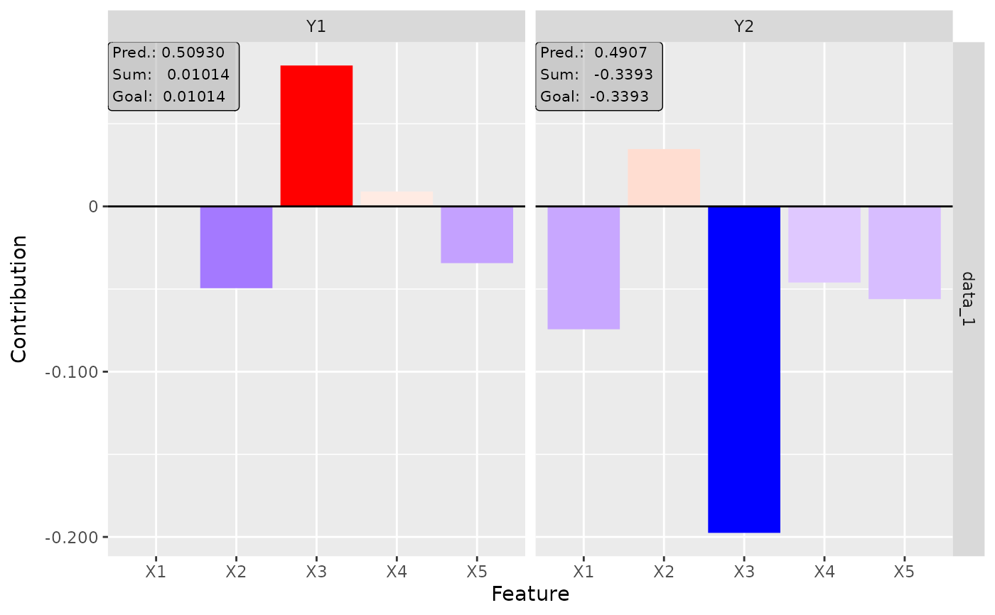
# Plot the result for both classes
plot(deepshap, output_idx = 1:2)
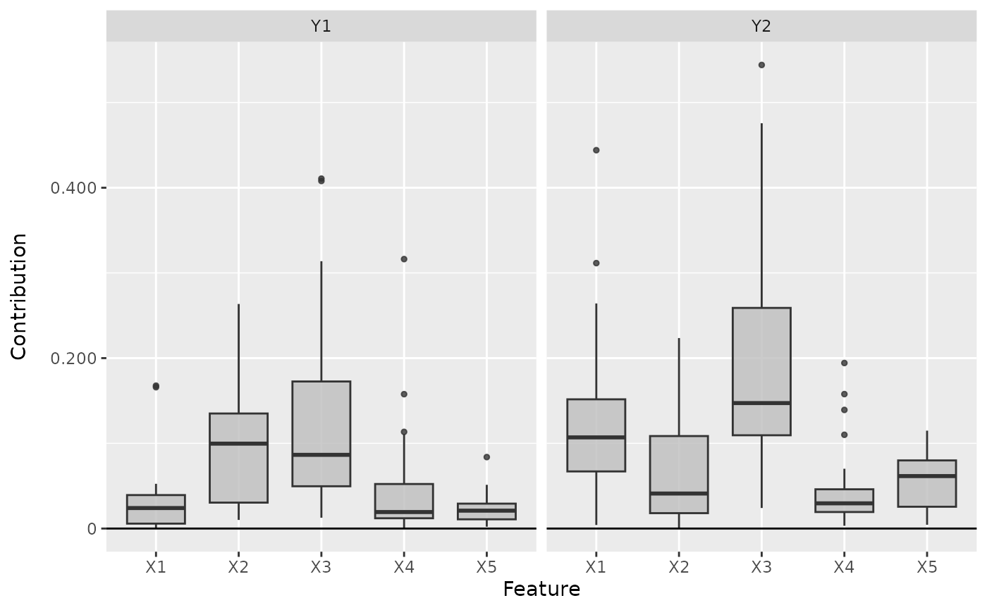
 # Plot the boxplot of all datapoints and for both classes
boxplot(deepshap, output_idx = 1:2)
# Plot the boxplot of all datapoints and for both classes
boxplot(deepshap, output_idx = 1:2)
 # ------------------------- Example 2: Neuralnet ---------------------------
if (require("neuralnet")) {
library(neuralnet)
data(iris)
# Train a neural network
nn <- neuralnet((Species == "setosa") ~ Petal.Length + Petal.Width,
iris,
linear.output = FALSE,
hidden = c(3, 2), act.fct = "tanh", rep = 1
)
# Convert the model
converter <- convert(nn)
# Apply DeepSHAP with rescale-rule and a 100 (default of `limit_ref`)
# instances as the reference dataset
deepshap <- run_deepshap(converter, iris[, c(3, 4)],
data_ref = iris[, c(3, 4)])
# Get the result as a dataframe and show first 5 rows
get_result(deepshap, type = "data.frame")[1:5, ]
# Plot the result for the first datapoint in the data
plot(deepshap, data_idx = 1)
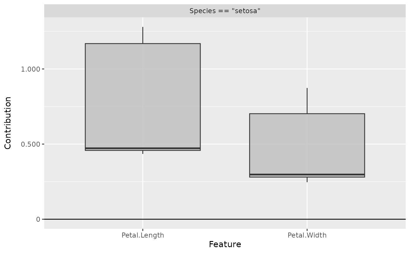
# Plot the result as boxplots
boxplot(deepshap)
}
# ------------------------- Example 2: Neuralnet ---------------------------
if (require("neuralnet")) {
library(neuralnet)
data(iris)
# Train a neural network
nn <- neuralnet((Species == "setosa") ~ Petal.Length + Petal.Width,
iris,
linear.output = FALSE,
hidden = c(3, 2), act.fct = "tanh", rep = 1
)
# Convert the model
converter <- convert(nn)
# Apply DeepSHAP with rescale-rule and a 100 (default of `limit_ref`)
# instances as the reference dataset
deepshap <- run_deepshap(converter, iris[, c(3, 4)],
data_ref = iris[, c(3, 4)])
# Get the result as a dataframe and show first 5 rows
get_result(deepshap, type = "data.frame")[1:5, ]
# Plot the result for the first datapoint in the data
plot(deepshap, data_idx = 1)
# Plot the result as boxplots
boxplot(deepshap)
}
 # ------------------------- Example 3: Keras -------------------------------
if (require("keras") & keras::is_keras_available()) {
library(keras)
# Make sure keras is installed properly
is_keras_available()
data <- array(rnorm(10 * 32 * 32 * 3), dim = c(10, 32, 32, 3))
model <- keras_model_sequential()
model %>%
layer_conv_2d(
input_shape = c(32, 32, 3), kernel_size = 8, filters = 8,
activation = "softplus", padding = "valid") %>%
layer_conv_2d(
kernel_size = 8, filters = 4, activation = "tanh",
padding = "same") %>%
layer_conv_2d(
kernel_size = 4, filters = 2, activation = "relu",
padding = "valid") %>%
layer_flatten() %>%
layer_dense(units = 64, activation = "relu") %>%
layer_dense(units = 16, activation = "relu") %>%
layer_dense(units = 2, activation = "softmax")
# Convert the model
converter <- convert(model)
# Apply the DeepSHAP method with zero baseline (wich is equivalent to
# DeepLift with zero baseline)
deepshap <- run_deepshap(converter, data, channels_first = FALSE)
# Plot the result for the first image and both classes
plot(deepshap, output_idx = 1:2)
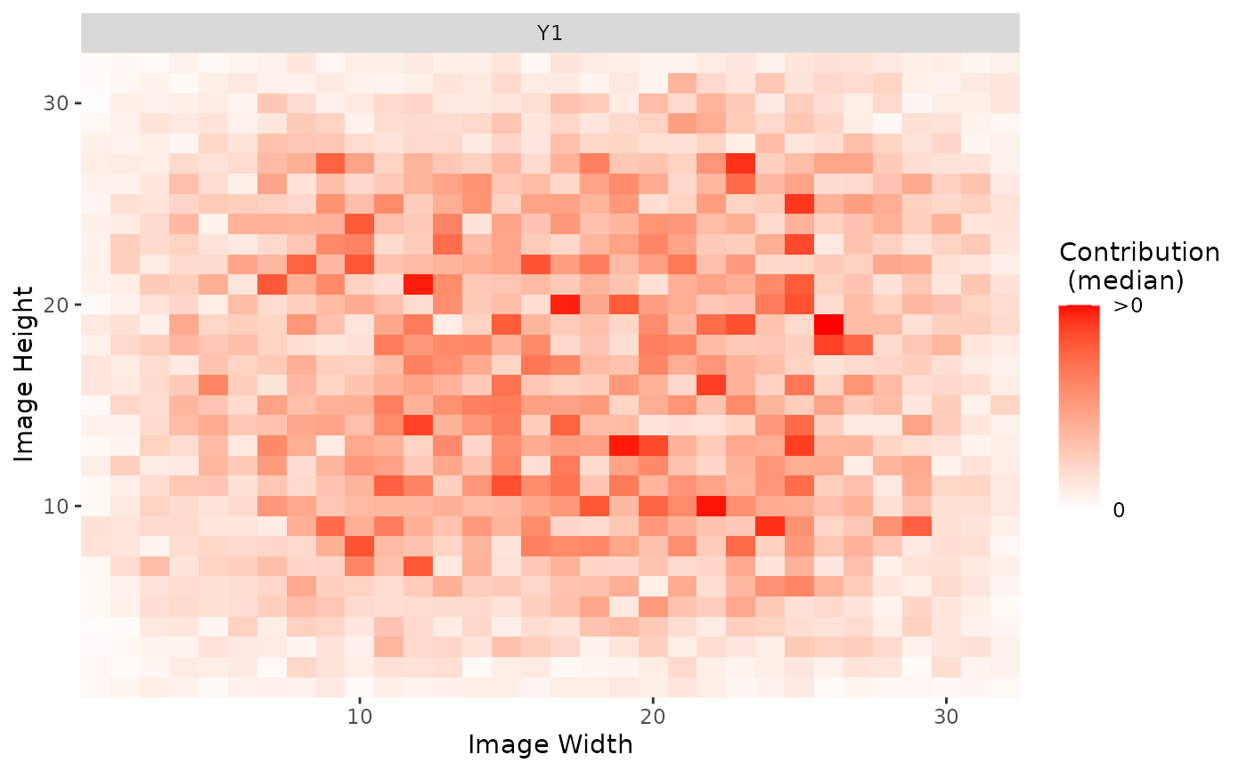
# Plot the pixel-wise median of the results
plot_global(deepshap, output_idx = 1)
}
# ------------------------- Example 3: Keras -------------------------------
if (require("keras") & keras::is_keras_available()) {
library(keras)
# Make sure keras is installed properly
is_keras_available()
data <- array(rnorm(10 * 32 * 32 * 3), dim = c(10, 32, 32, 3))
model <- keras_model_sequential()
model %>%
layer_conv_2d(
input_shape = c(32, 32, 3), kernel_size = 8, filters = 8,
activation = "softplus", padding = "valid") %>%
layer_conv_2d(
kernel_size = 8, filters = 4, activation = "tanh",
padding = "same") %>%
layer_conv_2d(
kernel_size = 4, filters = 2, activation = "relu",
padding = "valid") %>%
layer_flatten() %>%
layer_dense(units = 64, activation = "relu") %>%
layer_dense(units = 16, activation = "relu") %>%
layer_dense(units = 2, activation = "softmax")
# Convert the model
converter <- convert(model)
# Apply the DeepSHAP method with zero baseline (wich is equivalent to
# DeepLift with zero baseline)
deepshap <- run_deepshap(converter, data, channels_first = FALSE)
# Plot the result for the first image and both classes
plot(deepshap, output_idx = 1:2)
# Plot the pixel-wise median of the results
plot_global(deepshap, output_idx = 1)
}
 #------------------------- Plotly plots ------------------------------------
if (require("plotly")) {
# You can also create an interactive plot with plotly.
# This is a suggested package, so make sure that it is installed
library(plotly)
boxplot(deepshap, as_plotly = TRUE)
}
#> Warning: The `boxplot()` function is only intended for tabular or signal data. It is
#> called `plot_global()` instead.
#------------------------- Plotly plots ------------------------------------
if (require("plotly")) {
# You can also create an interactive plot with plotly.
# This is a suggested package, so make sure that it is installed
library(plotly)
boxplot(deepshap, as_plotly = TRUE)
}
#> Warning: The `boxplot()` function is only intended for tabular or signal data. It is
#> called `plot_global()` instead.