This class implements the Connection weights method investigated by Olden et al. (2004), which results in a relevance score for each input variable. The basic idea is to multiply all path weights for each possible connection between an input feature and the output node and then calculate the sum over them. Besides, it is originally a global interpretation method and independent of the input data. For a neural network with \(3\) hidden layers with weight matrices \(W_1\), \(W_2\) and \(W_3\), this method results in a simple matrix multiplication independent of the activation functions in between: $$W_1 * W_2 * W_3.$$
In this package, we extended this method to a local method inspired by the
method Gradient\(\times\)Input (see Gradient). Hence, the local variant is
simply the point-wise product of the global Connection weights method and
the input data. You can use this variant by setting the times_input
argument to TRUE and providing input data.
The R6 class can also be initialized using the run_cw function
as a helper function so that no prior knowledge of R6 classes is required.
References
J. D. Olden et al. (2004) An accurate comparison of methods for quantifying variable importance in artificial neural networks using simulated data. Ecological Modelling 178, p. 389–397
See also
Other methods:
DeepLift,
DeepSHAP,
ExpectedGradient,
Gradient,
IntegratedGradient,
LIME,
LRP,
SHAP,
SmoothGrad
Super class
innsight::InterpretingMethod -> ConnectionWeights
Public fields
times_input(
logical(1))
This logical value indicates whether the results from the Connection weights method were multiplied by the provided input data or not. Thus, this value specifies whether the original global variant of the method or the local one was applied. If the value isTRUE, then data is provided in the fielddata.
Methods
Method new()
Create a new instance of the class ConnectionWeights. When
initialized, the method is applied and the results
are stored in the field result.
Usage
ConnectionWeights$new(
  converter,
  data = NULL,
  output_idx = NULL,
  output_label = NULL,
  channels_first = TRUE,
  times_input = FALSE,
  verbose = interactive(),
  dtype = "float"
)
Arguments
converter(
Converter)
An instance of theConverterclass that includes the torch-converted model and some other model-specific attributes. SeeConverterfor details.data(
array,data.frame,torch_tensororlist)
The data to which the method is to be applied. These must have the same format as the input data of the passed model to the converter object. This means eitheran
array,data.frame,torch_tensoror array-like format of size (batch_size, dim_in), if e.g.the model has only one input layer, ora
listwith the corresponding input data (according to the upper point) for each of the input layers.
This argument is only relevant if
times_inputisTRUE, otherwise it will be ignored because it is a locale (i.e. explanation for each data point individually) method only in this case.output_idx(
integer,listorNULL)
These indices specify the output nodes for which the method is to be applied. In order to allow models with multiple output layers, there are the following possibilities to select the indices of the output nodes in the individual output layers:An
integervector of indices: If the model has only one output layer, the values correspond to the indices of the output nodes, e.g.,c(1,3,4)for the first, third and fourth output node. If there are multiple output layers, the indices of the output nodes from the first output layer are considered.A
listofintegervectors of indices: If the method is to be applied to output nodes from different layers, a list can be passed that specifies the desired indices of the output nodes for each output layer. Unwanted output layers have the entryNULLinstead of a vector of indices, e.g.,list(NULL, c(1,3))for the first and third output node in the second output layer.NULL(default): The method is applied to all output nodes in the first output layer but is limited to the first ten as the calculations become more computationally expensive for more output nodes.
output_label(
character,factor,listorNULL)
These values specify the output nodes for which the method is to be applied. Only values that were previously passed with the argumentoutput_namesin theconvertercan be used. In order to allow models with multiple output layers, there are the following possibilities to select the names of the output nodes in the individual output layers:A
charactervector orfactorof labels: If the model has only one output layer, the values correspond to the labels of the output nodes named in the passedConverterobject, e.g.,c("a", "c", "d")for the first, third and fourth output node if the output names arec("a", "b", "c", "d"). If there are multiple output layers, the names of the output nodes from the first output layer are considered.A
listofcharactor/factorvectors of labels: If the method is to be applied to output nodes from different layers, a list can be passed that specifies the desired labels of the output nodes for each output layer. Unwanted output layers have the entryNULLinstead of a vector of labels, e.g.,list(NULL, c("a", "c"))for the first and third output node in the second output layer.NULL(default): The method is applied to all output nodes in the first output layer but is limited to the first ten as the calculations become more computationally expensive for more output nodes.
channels_first(
logical(1))
The channel position of the given data (argumentdata). IfTRUE, the channel axis is placed at the second position between the batch size and the rest of the input axes, e.g.,c(10,3,32,32)for a batch of ten images with three channels and a height and width of 32 pixels. Otherwise (FALSE), the channel axis is at the last position, i.e.,c(10,32,32,3). If the data has no channel axis, use the default valueTRUE.times_input(
logical(1))
Multiplies the results with the input features. This variant turns the global Connection weights method into a local one. Default:FALSE.verbose(
logical(1))
This logical argument determines whether a progress bar is displayed for the calculation of the method or not. The default value is the output of the primitive R functioninteractive().dtype(
character(1))
The data type for the calculations. Use either'float'fortorch_floator'double'fortorch_double.
Examples
#----------------------- Example 1: Torch ----------------------------------
library(torch)
# Create nn_sequential model
model <- nn_sequential(
nn_linear(5, 12),
nn_relu(),
nn_linear(12, 1),
nn_sigmoid()
)
# Create Converter with input names
converter <- Converter$new(model,
input_dim = c(5),
input_names = list(c("Car", "Cat", "Dog", "Plane", "Horse"))
)
# You can also use the helper function for the initialization part
converter <- convert(model,
input_dim = c(5),
input_names = list(c("Car", "Cat", "Dog", "Plane", "Horse"))
)
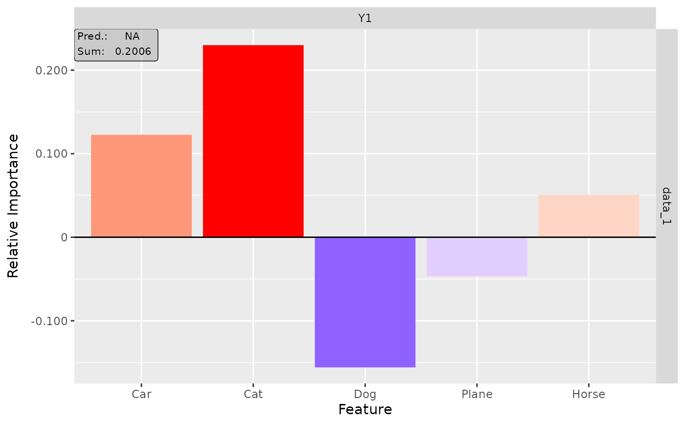
# Apply method Connection Weights
cw <- ConnectionWeights$new(converter)
# Again, you can use a helper function `run_cw()` for initializing
cw <- run_cw(converter)
# Print the head of the result as a data.frame
head(get_result(cw, "data.frame"), 5)
#> data model_input model_output feature output_node value pred
#> 1 data_1 Input_1 Output_1 Car Y1 -0.20152949 NA
#> 2 data_1 Input_1 Output_1 Cat Y1 0.26889324 NA
#> 3 data_1 Input_1 Output_1 Dog Y1 0.04307225 NA
#> 4 data_1 Input_1 Output_1 Plane Y1 0.08284904 NA
#> 5 data_1 Input_1 Output_1 Horse Y1 0.06484403 NA
#> decomp_sum decomp_goal input_dimension
#> 1 0.2581291 NA 1
#> 2 0.2581291 NA 1
#> 3 0.2581291 NA 1
#> 4 0.2581291 NA 1
#> 5 0.2581291 NA 1
# Plot the result
plot(cw)
 #----------------------- Example 2: Neuralnet ------------------------------
if (require("neuralnet")) {
library(neuralnet)
data(iris)
# Train a Neural Network
nn <- neuralnet((Species == "setosa") ~ Petal.Length + Petal.Width,
iris,
linear.output = FALSE,
hidden = c(3, 2), act.fct = "tanh", rep = 1
)
# Convert the trained model
converter <- convert(nn)
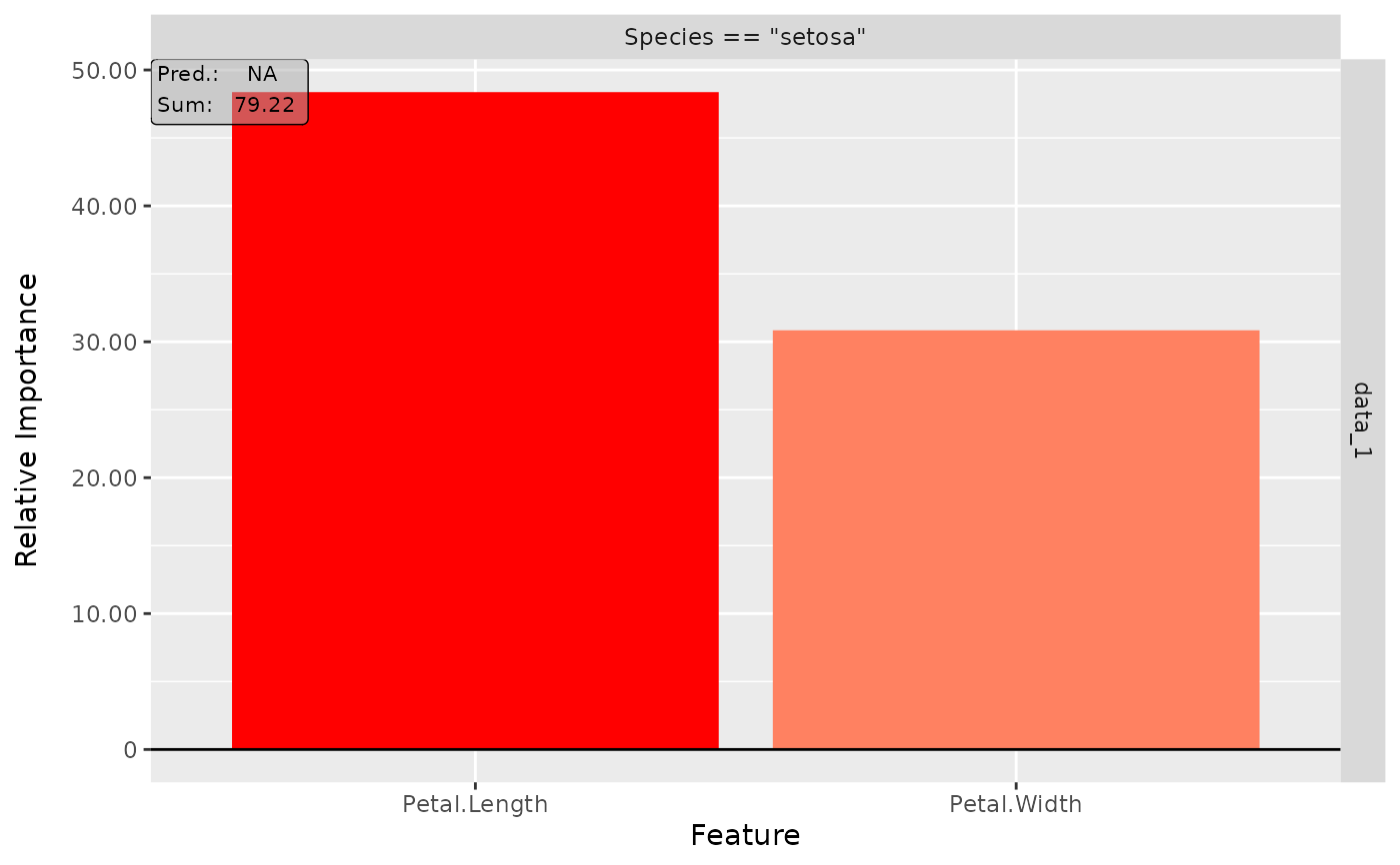
# Apply the Connection Weights method
cw <- run_cw(converter)
# Get the result as a torch tensor
get_result(cw, type = "torch.tensor")
# Plot the result
plot(cw)
}
#> Loading required package: neuralnet
#----------------------- Example 2: Neuralnet ------------------------------
if (require("neuralnet")) {
library(neuralnet)
data(iris)
# Train a Neural Network
nn <- neuralnet((Species == "setosa") ~ Petal.Length + Petal.Width,
iris,
linear.output = FALSE,
hidden = c(3, 2), act.fct = "tanh", rep = 1
)
# Convert the trained model
converter <- convert(nn)
# Apply the Connection Weights method
cw <- run_cw(converter)
# Get the result as a torch tensor
get_result(cw, type = "torch.tensor")
# Plot the result
plot(cw)
}
#> Loading required package: neuralnet
 # ------------------------- Example 3: Keras -------------------------------
if (require("keras") & keras::is_keras_available()) {
library(keras)
# Make sure keras is installed properly
is_keras_available()
data <- array(rnorm(10 * 32 * 32 * 3), dim = c(10, 32, 32, 3))
model <- keras_model_sequential()
model %>%
layer_conv_2d(
input_shape = c(32, 32, 3), kernel_size = 8, filters = 8,
activation = "softplus", padding = "valid") %>%
layer_conv_2d(
kernel_size = 8, filters = 4, activation = "tanh",
padding = "same") %>%
layer_conv_2d(
kernel_size = 4, filters = 2, activation = "relu",
padding = "valid") %>%
layer_flatten() %>%
layer_dense(units = 64, activation = "relu") %>%
layer_dense(units = 16, activation = "relu") %>%
layer_dense(units = 2, activation = "softmax")
# Convert the model
converter <- convert(model)
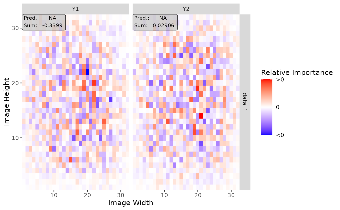
# Apply the Connection Weights method
cw <- run_cw(converter)
# Get the head of the result as a data.frame
head(get_result(cw, type = "data.frame"), 5)
# Plot the result for all classes
plot(cw, output_idx = 1:2)
}
#> Loading required package: keras
#> The keras package is deprecated. Please use the keras3 package instead.
#> Alternatively, to continue using legacy keras, call `py_require_legacy_keras()`.
# ------------------------- Example 3: Keras -------------------------------
if (require("keras") & keras::is_keras_available()) {
library(keras)
# Make sure keras is installed properly
is_keras_available()
data <- array(rnorm(10 * 32 * 32 * 3), dim = c(10, 32, 32, 3))
model <- keras_model_sequential()
model %>%
layer_conv_2d(
input_shape = c(32, 32, 3), kernel_size = 8, filters = 8,
activation = "softplus", padding = "valid") %>%
layer_conv_2d(
kernel_size = 8, filters = 4, activation = "tanh",
padding = "same") %>%
layer_conv_2d(
kernel_size = 4, filters = 2, activation = "relu",
padding = "valid") %>%
layer_flatten() %>%
layer_dense(units = 64, activation = "relu") %>%
layer_dense(units = 16, activation = "relu") %>%
layer_dense(units = 2, activation = "softmax")
# Convert the model
converter <- convert(model)
# Apply the Connection Weights method
cw <- run_cw(converter)
# Get the head of the result as a data.frame
head(get_result(cw, type = "data.frame"), 5)
# Plot the result for all classes
plot(cw, output_idx = 1:2)
}
#> Loading required package: keras
#> The keras package is deprecated. Please use the keras3 package instead.
#> Alternatively, to continue using legacy keras, call `py_require_legacy_keras()`.
 #------------------------- Plotly plots ------------------------------------
if (require("plotly")) {
# You can also create an interactive plot with plotly.
# This is a suggested package, so make sure that it is installed
library(plotly)
plot(cw, as_plotly = TRUE)
}
#> Loading required package: plotly
#> Loading required package: ggplot2
#>
#> Attaching package: ‘plotly’
#> The following object is masked from ‘package:ggplot2’:
#>
#> last_plot
#> The following object is masked from ‘package:stats’:
#>
#> filter
#> The following object is masked from ‘package:graphics’:
#>
#> layout
#------------------------- Plotly plots ------------------------------------
if (require("plotly")) {
# You can also create an interactive plot with plotly.
# This is a suggested package, so make sure that it is installed
library(plotly)
plot(cw, as_plotly = TRUE)
}
#> Loading required package: plotly
#> Loading required package: ggplot2
#>
#> Attaching package: ‘plotly’
#> The following object is masked from ‘package:ggplot2’:
#>
#> last_plot
#> The following object is masked from ‘package:stats’:
#>
#> filter
#> The following object is masked from ‘package:graphics’:
#>
#> layout