In-depth explanation

📝 Note
Since the innsight package relies on the torch package for each method and this requires a successful installation of LibTorch and other dependencies (torch::install_torch()), no examples can be run in the R vignette for memory reasons. For the executed code chunks, we refer to our website.

As described in the introduction, innsight is a package that aims to be highly flexible and easily accessible to almost any R user from any background. This vignette describes in detail all the possibilities to explain a prediction of a data instance for a given model using the provided methods and how to create a visualization of the results.

Step 1: The Converter

The R6 class Converter is the heart of the package and makes it to a deep-learning-model-agnostic approach, i.e., it accepts models not only from a single deep learning library but from many different libraries. This property makes the package outstanding and highly flexible. Internally, each layer is analyzed, and the relevant parameters and components are extracted into a list. Afterward, a customized model based on the library torch is generated from this list, with the interpretation methods pre-implemented in each of the accepted layers and modules. On this baseline, different methods can be implemented and applied later in step 2. To be able to create a new object, the following call is used:

converter <- Converter$new(model,
  input_dim = NULL,
  input_names = NULL,
  output_names = NULL,
  dtype = "float",
  save_model_as_list = FALSE
)

As you can see, the Converter class is implemented using an R6::R6Class() class. However, this assumes that users have prior knowledge of these classes, potentially making the application a bit unfamiliar. For this reason, we have implemented a shortcut function that initializes an object of the Converter class in a more familiar R syntax:

converter <- convert(model,
  input_dim = NULL,
  input_names = NULL,
  output_names = NULL,
  dtype = "float",
  save_model_as_list = FALSE
)

Argument model

This is the passed trained model. Currently, it can be a sequential torch model (nn_sequential()), a tensorflow/keras model (keras_model() or keras_model_sequential()), a neuralnet model or a model as a list. All these options are explained in detail in the following subsections.

Package torch

Currently, only models created by torch::nn_sequential are accepted. However, the most popular standard layers and activation functions are available:

• Linear layers: nn_linear()

• Convolutional layers: nn_conv1d(), nn_conv2d() (but only with padding_mode = "zeros" and numerical padding)

• Max-pooling layers: nn_max_pool1d(), nn_max_pool2d() (both only with default arguments for padding = 0, dilation = 1, return_indices = FALSE and ceil_mode = FALSE)

• Average-pooling layers: nn_avg_pool1d(), nn_avg_pool2d() (both only with default arguments for padding = 0, return_indices = FALSE and ceil_mode = FALSE)

• Batch-normalization layers: nn_batch_norm1d(), nn_batch_norm2d()

• Flatten layer: nn_flatten()

• Skipped layers: nn_dropout()

• Activation functions: nn_relu, nn_leaky_relu, nn_softplus, nn_sigmoid, nn_softmax, nn_tanh (open an issue if you need any more)

📝 Notes

In a torch model, the shape of the inputs is not stored; hence it must be specified with the argument input_dim within the initialization of the Converter object.

Example: Convert a torch model

library(torch)

torch_model <- nn_sequential(
  nn_conv2d(3, 5, c(2, 2), stride = 2, padding = 3),
  nn_relu(),
  nn_avg_pool2d(c(2, 2)),
  nn_flatten(),
  nn_linear(80, 32),
  nn_relu(),
  nn_dropout(),
  nn_linear(32, 2),
  nn_softmax(dim = 2)
)

# For torch models the optional argument `input_dim` becomes a necessary one
converter <- convert(torch_model, input_dim = c(3, 10, 10))
#> Skipping nn_dropout ...

Package keras

Keras models created by keras_model_sequential or keras_model are accepted. Within these functions, the following layers are allowed to be used:

• Input layer: layer_input()

• Linear layers: layer_dense()

• Convolutional layers: layer_conv_1d(), layer_conv_2d()

• Pooling layers: layer_max_pooling_1d(), layer_max_pooling_2d(), layer_average_pooling_1d(), layer_average_pooling_2d(), layer_global_average_pooling_1d(), layer_global_average_pooling_2d(), layer_global_max_pooling_1d(), layer_global_max_pooling_2d()

• Batch-normalization layer: layer_batch_normalization()

• Flatten layer: layer_flatten()

• Merging layers: layer_add(), layer_concatenate() (but it is assumed that the concatenation axis points to the channel axis)

• Padding layers: layer_zero_padding_1d(), layer_zero_padding_2d()

• Skipped layers: layer_dropout()

• Activation functions: The following activation functions are allowed as character argument (activation) in a linear and convolutional layer: "relu", "softplus", "sigmoid", "softmax", "tanh", "linear". But you can also specify the activation function as a standalone layer: layer_activation_relu(), layer_activation_softmax(). But keep in mind that an activation layer may only follow a dense, convolutional or pooling layer. If you miss an activation function, feel free to open an issue on GitHub.

Examples: Convert a keras model

Example 1: keras_model_sequential

library(keras)

# Create model
keras_model_seq <- keras_model_sequential()
keras_model_seq <- keras_model_seq %>%
  layer_dense(10, input_shape = c(5), activation = "softplus") %>%
  layer_dense(8, use_bias = FALSE, activation = "tanh") %>%
  layer_dropout(0.2) %>%
  layer_dense(4, activation = "softmax")

converter <- convert(keras_model_seq)
#> Skipping Dropout ...

Example 2: keras_model

library(keras)

input_image <- layer_input(shape = c(10, 10, 3))
input_tab <- layer_input(shape = c(20))

conv_part <- input_image %>%
  layer_conv_2d(5, c(2, 2), activation = "relu", padding = "same") %>%
  layer_average_pooling_2d() %>%
  layer_conv_2d(4, c(2, 2)) %>%
  layer_activation(activation = "softplus") %>%
  layer_flatten()

output <- layer_concatenate(list(conv_part, input_tab)) %>%
  layer_dense(50, activation = "relu") %>%
  layer_dropout(0.3) %>%
  layer_dense(3, activation = "softmax")

keras_model_concat <- keras_model(inputs = list(input_image, input_tab), outputs = output)

converter <- convert(keras_model_concat)
#> Skipping InputLayer ...
#> Skipping InputLayer ...
#> Skipping Dropout ...

Package neuralnet

Using nets from the package neuralnet is very simple and straightforward, because the package offers much fewer options than torch or keras. The only thing to note is that no custom activation function can be used. However, the package saves the names of the inputs and outputs, which can, of course, be overwritten with the arguments input_names and output_names when creating the converter object.

Example: Convert a neuralnet model

library(neuralnet)
data(iris)
set.seed(42)

# Create model
neuralnet_model <- neuralnet(Species ~ Petal.Length + Petal.Width, iris,
  linear.output = FALSE
)

# Convert model
converter <- convert(neuralnet_model)
# Show input names
converter$input_names
#> [[1]]
#> [[1]][[1]]
#> [1] Petal.Length Petal.Width 
#> Levels: Petal.Length Petal.Width
# Show output names
converter$output_names
#> [[1]]
#> [[1]][[1]]
#> [1] setosa     versicolor virginica 
#> Levels: setosa versicolor virginica

Model as named list

Besides models from the packages keras, torch and neuralnet it is also possible to pass a self-defined model in the form of a named list to the Converter class/convert() function. This enables the interpretation of networks from other libraries with all available methods provided by the innsight package.

If you want to create a custom model, your list (e.g., model <- list()) needs at least the keys model$input_dim and model$layers. However, other optional keys that can be used to name the input features and output nodes or to test the model for correctness. In summary:

• input_dim
  The model input dimension excluding the batch dimension in the format “channels first”. If there is only one input layer, it can be specified as a vector. Otherwise, use a list of the shapes of the individual input layers in the correct order.

  Examples

  1. one dense input layer with five features:

  model$input_dim <- c(5)

  2. two input layers consisting of one dense layer of shape $10$ and one convolutional layer of shape $10\times10\times3$:

  input_dim <- list(c(10), c(3, 10, 10)) # channels have to be first!

  
  
• input_nodes
  An integer vector specifying the indices of the input layers from the layers list. If there are multiple input layers, the indices of the corresponding layers must be in the same order as in the input_dim and input_names arguments. If this argument is not set, a warning is printed and it is assumed that the first layer in layers is the only input layer.
  
  

• input_names (optional)
  The names for each input dimension excluding the batch axis in the format “channels first”. If there is only one input layer, it can be specified as a list of character vectors or factors for each input axis. Otherwise, use a list of those for each input layer in the correct order.

  Examples

  1. one dense layer with two features:

  model$input_names <- c("Feature_1", "Feature_2")

  2. one convolutional layer with shape $3\times 3\times 2$:

  model$input_names <- list(c("C1", "C2"), c("H1", "H2"), c("W1", "W2"))

  3. two input layers consisting of one dense layer of shape $2$ and one convolutional layer of shape $3\times3\times2$:

  model$input_names <- list(
    list(c("Feature_1", "Feature_2")),
    list(c("C1", "C2"), c("H1", "H2"), c("W1", "W2"))
  )

• output_dim (optional)
  An integer vector or a list of vectors with the model output dimension without the batch dimension analogous to input_dim. This value does not need to be specified and will be calculated otherwise. However, if it is set, the calculated value will be compared with it to avoid errors while converting the model.

• output_nodes
  An integer vector specifying the indices of the output layers from the layers list. If there are multiple output layers, the indices of the corresponding layers must be in the same order as in the output_dim and output_names arguments. If this argument is not set, a warning is printed and it is assumed that the last layer in layers is the only output layer.
  
  

• output_names (optional)
  A list or a list of lists with the names for each output dimension for each output layer analogous to input_names. By default (NULL), the names are generated.

• layers
  (see next subsection)

📝 Notes
The arguments for the input and output names are optional. By default (NULL), they are generated, i.e.,

• the output names are c("Y1", "Y2", "Y3", ... ) for each output layer.

• the input names are

  • c("X1", "X2", "X3", ...) for tabular input layers,
    
  • list(c("C1", "C2", ...), c("L1", "L2", ...)) for 1D input layers and
    
  • list(c("C1", "C2", ...), c("H1", "H2", ...), c("W1", "W2", ...)) for 2D input layers.

Adding layers to your list-model

The list entry layers contains a list with all accepted layers of the model. In general, each element has the following three arguments:

• type: The type of the layer, e.g., "Dense", "Conv2D", "MaxPooling1D", etc. (see blow for all accepted types).

• input_layers: The list indices from the layers list going into this layer, i.e., the previous layers. If this argument is not set, a warning is printed and it is assumed that the previous list index in layers is the only preceding layer. If this layer is an input layer, use the value 0.

• output_layers: The list indices from the layers list that follow this layer. If this argument is not set, a warning is printed and it is assumed that the next list index in layers is the only following layer. If this layer is an output layer, use the value -1.

• dim_in (optional): The input dimension of this layer excluding the batch axis according to the format

  • $\left( \text{feat}_\text{in} \right)$ for tabular data, e.g., c(3) for $3$ features,

  • $\left(\text{channels}_\text{in}, \text{length}_\text{in} \right)$ for 1D signal data, e.g., c(3,10) for signals with length $10$ and $3$ channels or

  • $\left(\text{channels}_\text{in}, \text{height}_\text{in}, \text{width}_\text{in} \right)$ for 2D image data, e.g., c(3,10,10) for images of shape $10\times10$ with $3$ channels.

  • For merging layers, a list of the above formats is required, but this is described in more detail in the corresponding types below.

  This value is not necessary, but helpful to check the format of the weight matrix and the overall correctness of the converted model.

• dim_out (optional): The output dimension of this layer excluding the batch axis analogous to the argument dim_in. This value is not necessary, but helpful to check the format of the weight matrix and the overall correctness of the converted model.

In addition to these main arguments, individual arguments can be set for each layer type, as described below:

Dense layer (type = "Dense")

• weight: The weight matrix of the dense layer with shape (dim_out, dim_in).

• bias: The bias vector of the dense layer with length dim_out.

• activation_name: The name of the activation function for this dense layer, e.g., 'linear', 'relu', 'tanh' or 'softmax'.

Example for a dense layer

# Define dense layer
dense_layer <- list(
  type = "Dense",
  input_layers = 0, # '0' means input layer
  output_layers = 2,
  weight = matrix(rnorm(5 * 2), 2, 5),
  bias = rnorm(2),
  activation_name = "tanh",
  dim_in = 5, # optional
  dim_out = 2 # optional
)

Convolutional layer (type = "Con1D" or "Con2D")

• weight: The weight array of the convolutional layer with shape $\left(\text{channels}_\text{out}, \text{channels}_\text{in}, \text{kernel}_\text{length}\right)$ for 1D signal or $\left(\text{channels}_\text{out}, \text{channels}_\text{in}, \text{kernel}_\text{height}, \text{kernel}_\text{width}\right)$ for 2D image.

• bias: The bias vector of the layer with length $\text{channels}_\text{out}$.

• activation_name: The name of the activation function for this layer, e.g., 'linear', 'relu', 'tanh' or 'softmax'.

• stride (optional): The stride of the convolution (single integer for 1D and tuple of two integers for 2D data). If this value is not specified, the default values (1D: 1 and 2D: c(1,1)) are used.

• padding (optional): Zero-padding added to the sides of the input before convolution. For 1D-convolution a tuple of the form $\left(\text{pad}_\text{left}, \text{pad}_\text{right}\right)$ and for 2D-convolution $\left(\text{pad}_\text{left}, \text{pad}_\text{right}, \text{pad}_\text{top}, \text{pad}_\text{bottom}\right)$ is required. If this value is not specified, the default values (1D: c(0,0) and 2D: c(0,0,0,0)) are used.

• dilation (optional): Spacing between kernel elements (single integer for 1D and tuple of two integers for 2D data). If this value is not specified, the default values (1D: 1 and 2D: c(1,1)) are used.

Examples for convolutional layers

# 1D convolutional layer
conv_1D <- list(
  type = "Conv1D",
  input_layers = 1,
  output_layers = 3,
  weight = array(rnorm(8 * 3 * 2), dim = c(8, 3, 2)),
  bias = rnorm(8),
  padding = c(2, 1),
  activation_name = "tanh",
  dim_in = c(3, 10), # optional
  dim_out = c(8, 9) # optional
)

# 2D convolutional layer
conv_2D <- list(
  type = "Conv2D",
  input_layes = 3,
  output_layers = 5,
  weight = array(rnorm(8 * 3 * 2 * 4), dim = c(8, 3, 2, 4)),
  bias = rnorm(8),
  padding = c(1, 1, 0, 0),
  dilation = c(1, 2),
  activation_name = "relu",
  dim_in = c(3, 10, 10) # optional
)

Pooling layer (type = "MaxPooling1D", "MaxPooling2D", "AveragePooling1D" or "AveragePooling2D")

• kernel_size: The size of the pooling window as an integer value for 1D-pooling and an tuple of two integers for 2D-pooling.

• strides (optional): The stride of the pooling window (single integer for 1D and tuple of two integers for 2D data). If this value is not specified (NULL), the value of kernel_size will be used.

Example for a pooling layer

# 2D average pooling layer
avg_pool2D <- list(
  type = "AveragePooling2D",
  input_layers = 1,
  output_layers = 3,
  kernel_size = c(2, 2)
)

Batch-Normalization layer (type = "BatchNorm")

During inference, the layer normalizes its output using a moving average of the mean and standard deviation of the batches it has seen during training, i.e., $$y = \gamma \cdot \frac{x - \mu}{\sqrt{\sigma + \varepsilon}} + \beta$$

• num_features: The number of features to normalize over. Usually the number of channels is used.

• eps: The value $\varepsilon$ added to the denominator for numerical stability.

• gamma: The vector of scaling factors $\gamma$ for each feature to be normalized, i.e., a numerical vector of length num_features.

• beta: The vector of offset values $\beta$ for each feature to be normalized, i.e., a numerical vector of length num_features.

• run_mean: The vector of running means $\mu$ for each feature to be normalized, i.e., a numerical vector of length num_features.

• run_var: The vector of running variances $\sigma$ for each feature to be normalized, i.e., a numerical vector of length num_features.

Example for a batch normalization layer

# batch normalization layer
batchnorm <- list(
  type = "BatchNorm",
  input_layers = 1,
  output_layers = 3,
  num_features = 3,
  eps = 1e-4,
  gamma = c(1.1, 0.0, -0.3),
  beta = c(1, -3, -1.4),
  run_mean = c(-1.9, 3, 2.3),
  run_var = c(1, 2.1, 3.5)
)

Flatten layer (type = "Flatten")

• start_dim (optional): An integer value that describes the axis from which the dimension is flattened. By default (NULL) the axis following the batch axis is selected, i.e., 2.

• end_dim (optional): An integer value that describes the axis to which the dimension is flattened. By default (NULL) the last axis is selected, i.e., -1.

Example for a flatten layer

# flatten layer
flatten <- list(
  type = "Flatten",
  input_layers = 1,
  output_layers = 3,
  start_dim = 2, # optional
  end_dim = 4, # optional
  dim_in = c(3, 10, 10), # optional
  out_dim = c(300) # optional
)

Global pooling layer (type = "GlobalPooling")

• method: Use either 'average' for global average pooling or 'max' for global maximum pooling.

Examples for global pooling layers

# global MaxPooling layer
global_max_pool2D <- list(
  type = "GlobalPooling",
  input_layers = 1,
  output_layers = 3,
  method = "max",
  dim_in = c(3, 10, 10), # optional
  out_dim = c(3) # optional
)

# global AvgPooling layer
global_avg_pool1D <- list(
  type = "GlobalPooling",
  input_layers = 1,
  output_layers = 3,
  method = "average",
  dim_in = c(3, 10), # optional
  out_dim = c(3) # optional
)

Padding layer (type = "Padding")

• padding: This integer vector specifies the number of padded elements, but its length depends on the input size:

  • length of 2 for 1D signal data: $\left(\text{pad}_\text{left}, \text{pad}_\text{right}\right)$
  • length of 4 for 2D image data: $\left(\text{pad}_\text{left}, \text{pad}_\text{right}, \text{pad}_\text{top}, \text{pad}_\text{bottom} \right)$.

• mode: The padding mode. Use either 'constant' (default), 'reflect', 'replicate' or 'circular'.

• value: The fill value for 'constant' padding.

Example for a padding layer

# padding layer
padding <- list(
  type = "Padding",
  input_layers = 1,
  output_layers = 3,
  padding = c(2, 4),
  mode = "constant",
  value = 1,
  dim_in = c(3, 10), # optional
  out_dim = c(3, 16) # optional
)

Concatenation layer (type = "Concatenate")

• dim: An integer value that describes the axis over which the inputs are concatenated.

📝 Note
For this layer the argument dim_in is a list of input dimensions.

Example for a concatenation layer

# concatenation layer
concat <- list(
  type = "Concatenation",
  input_layers = c(1, 3),
  output_layers = 5,
  dim = 2,
  dim_in = list(c(5), c(3)), # optional
  out_dim = c(8) # optional
)

Adding layer (type = "Add")

📝 Note
For this layer the argument dim_in is a list of input dimensions.

Example for an adding layer

# adding layer
add <- list(
  type = "Add",
  input_layers = c(1, 3),
  output_layers = 5,
  dim_in = list(c(3, 10, 10), c(3, 10, 10)), # optional
  out_dim = c(3, 10, 10) # optional
)

Argument input_dim

With the argument input_dim, input size excluding the batch dimension is passed. For many packages, this information is already included in the given model. In this case, this argument only acts as a check and throws an error in case of inconsistency. However, if the input size is not included in the model, which is, for example, the case for models from the package torch, it becomes a necessary argument and the correct size must be passed. All in all, four different forms of input shapes are accepted, whereby all shapes with channels must always be in the “channels first” format for internal reasons:

• Tabular inputs: If the model has no channels and is only one-dimensional, the input size can be passed as a single integer or vector with a single integer, e.g., a dense layer with five features would have an input shape of 5 or c(5).

• Signal inputs: If the model has signals consisting of a channel and another dimension as input, the input size can be passed as a vector composed of the number of channels $C$ and the signal length $L$ in the channels first format, i.e., $\left(C, L\right)$. For example, for a 1D convolutional layer with three channels and a signal length of $10$ (both formats $3 \times 10$ and $10 \times 3$), the shape c(3, 10) must be passed.

• Image inputs: If the model has images consisting of a channel and two other dimensions as input, the input size can be passed as a vector composed of the number of channels $C$, the image height $H$ and width $W$ in the channels first format, i.e., $\left(C, H, W\right)$. For example, for a 2D convolutional layer with three channels, image height of $32$ and width of $20$ (both formats $3 \times 32 \times 20$ and $32 \times 20 \times 3$), the shape c(3, 32, 20) must be passed.

• Multiple inputs: If the passed model has multiple input layers, they can be passed in the correct layer-order in a list of the shapes from above. For example, for a model with an input layer with five features and another input layer with images of size $32\times32\times3$, the list list(c(5), c(3, 32, 32)) must be passed.

  📝 Note
  With multiple input layers, it is required that the original ordering of the input layers of the passed model matches the ordering in input_dim and also the ordering of the input names in the input_names argument.

Argument input_names

According to the shapes from the argument input_dim, the input names for each layer and dimension can be passed with the optional argument input_names. This means that for each integer in input_dim a vector of this length is passed with the labels, which is then summarized for all dimensions in a list. The labels can be provided both as normal character vectors and as factors and they will be used for the visualizations in Step 3. Factors can be used to specify the order of the labels as they will be visualized later in Step 3. For the individual input formats, the input names can be passes as described below:

• Tabular inputs: If, for example, input_dim = c(4), a possible value for the input names can be

  list(c("set", "your", "labels", "here!"))
  # or as a factor
  list(
    factor(c("set", "your", "labels", "here"),
      levels = c("labels", "set", "your", "here")
    )
  )

• Signal inputs: If, for example, input_dim = c(3, 6), a possible value for the input names can be

  list(
    c("channels", "are", "first"),
    c("Length1", "Length2", "Length3", "Length4", "Length5", "Length6")
  )

• Image inputs: If, for example, input_dim = c(3, 4, 4), a possible value for the input names can be

  list(
    c("channels", "are", "first"),
    c("then", "comes", "the", "image height"),
    c("and", "then", "the", "width")
  )

• Multiple inputs: If, for example, input_dim = list(c(4), c(3, 4, 4)), a possible value for the input names can be

  list(
    # first input layer
    list(c("Feat_1", "Feat_2", "Feat_3", "Feat_4")),
    # second input layer
    list(
      c("C1", "C2", "C3"),
      c("Height_1", "Height_2", "Height_3", "Height_4"),
      c("W1", "W2", "W3", "W4")
    )
  )

📝 Notes
The argument for the input names is optional. By default (NULL) they are generated, i.e., the input names are

• list(c("X1", "X2", "X3", ...)) for tabular input layers
• list(c("C1", "C2", ...), c("L1", "L2", ...)) for 1D input layers
• list(c("C1", "C2", ...), c("H1", "H2", ...), c("W1", "W2", ...)) for 2D input layers.

Argument output_names

The optional argument output_names can be used to define the names of the outputs for each output layer analog to input_names for the inputs. During the initialization of the Converter instance, the output size is calculated and stored in the field output_dim, which is structured in the same way as the argument input_dim. This results in the structure of the argument output_names analogous to the argument input_names, i.e., a vector of labels, a factor or, in case of several output layers, a list of label vectors or factors. For example, for an output layer with three nodes, the following list of labels can be passed:

c("First output node", "second one", "last output node")
# or as a factor
factor(c("First output node", "second one", "last output node"),
  levels = c("last output node", "First output node", "second one", )
)

For a model with two output layers (two nodes in the first and four in the second), the following input would be valid:

list(
  c("Yes", "No!"),
  c("Out1", "Out2", "Out3", "Out4")
)

Since it is an optional argument, the labels c("Y1", "Y2", "Y3", ...) are generated with the default value NULL for each output layer.

Other arguments

Argument dtype

This argument defines the numerical floating-point number’s precision with which all internal calculations are performed. Accepted are currently 32-bit floating point ("float" the default value) and 64-bit floating point numbers ("double"). All weights, constants and inputs are then converted accordingly into the data format torch_float() or torch_double().

📝 Note
At this point, this decision is especially crucial for exact comparisons, and if the precision is too inaccurate, errors could occur. See the following example:

Example

We create two random $10 \times 10$ matrices $A$ and $B$:

torch_manual_seed(123)
A <- torch_randn(10, 10)
B <- torch_randn(10, 10)

Now it can happen that the results of functions like torch_mm and a manual calculation differ:

# result of first row and first column after matrix multiplication
res1 <- torch_mm(A, B)[1, 1]
# calculation by hand
res2 <- sum(A[1, ] * B[, 1])

# difference:
res1 - res2
#> torch_tensor
#> -2.38419e-07
#> [ CPUFloatType{} ]

This is an expected behavior, which is explained in detail in the PyTorch documentation here. But you can reduce the error by using the double precision with torch_double():

torch_manual_seed(123)
A <- torch_randn(10, 10, dtype = torch_double())
B <- torch_randn(10, 10, dtype = torch_double())

# result of first row and first column after matrix multiplication
res1 <- torch_mm(A, B)[1, 1]
# calculation by hand
res2 <- sum(A[1, ] * B[, 1])

# difference:
res1 - res2
#> torch_tensor
#> 0
#> [ CPUDoubleType{} ]

Argument save_model_as_list

As already described in the introduction vignette, a given model is first converted to a list and then the torch model is created from it. By default, however, this list is not stored in the Converter object, since this requires a lot of memory for large models and is otherwise not used further. With the logical argument save_model_as_list, this list can be stored in the field model_as_list for further investigations. For example, this list can again be used as a model for a new Converter instance.

Fields

After an instance of the Converter class has been successfully created, the most important arguments and results are stored in the fields of the R6 object. The existing fields are explained briefly in the following:

• model: This field contains the torch-converted model based on the module ConvertedModel (see ?ConvertedModel for more information) containing the model with pre-implemented feature attribution methods.

• input_dim: This field is more or less a copy of the argument input_dim of the Converter object, only unified that it is always a list of the input shapes for each input layer, i.e., the argument input_dim = c(4) turns into list(c(4)).

• input_names: Analog to the field input_dim, the field input_names contains the input labels of the Converter argument input_names, but as a list of the label lists for each input layer, i.e., the argument input_names = list(c("C1", "C2"), c("A", "B")) turns into list(list(c("C1", "C2"), c("A", "B"))).

• output_dim: This field contains a list of the calculated output shapes of each output layer.

• output_names: Analog to the field input_names but for the argument output_names.

• model_as_list: The given model converted to a list (see argument save_model_as_list for more information).

Examples: Accessing and working with fields

Let’s consider again the model from Example 2 in the keras section (make sure that the model keras_model_concat is loaded!):

# Convert the model and save the model as a list
converter <- convert(keras_model_concat, save_model_as_list = TRUE)
#> Skipping InputLayer ...
#> Skipping InputLayer ...
#> Skipping Dropout ...

# Get the field `input_dim`
converter$input_dim
#> [[1]]
#> [1]  3 10 10
#> 
#> [[2]]
#> [1] 20

As you can see, the model has two input layers. The first one is for images of shape $3 \times 10 \times 10$ and the second layer for dense inputs of shape $20$. For example, we can now examine whether the converted model provides the same output as the original model:

# create input in the format "channels last"
x <- list(
  array(rnorm(3 * 10 * 10), dim = c(1, 10, 10, 3)),
  array(rnorm(20), dim = c(1, 20))
)

# output of the original model
y_true <- as.array(keras_model_concat(x))
# output of the torch-converted model (the data 'x' is in the format channels
# last, hence we need to set the argument 'channels_first = FALSE')
y <- as.array(converter$model(x, channels_first = FALSE)[[1]])

# mean squared error
mean((y - y_true)**2)
#> [1] 1.184238e-15

Since we did not pass any arguments for the input and output names, they were generated and stored in the list format in the input_names and output_names fields. Remember that in these fields, regardless of the number of input or output layers, there is always an outer list for the layers and then inner lists for the layer’s dimensions.

# get the calculated output dimension
str(converter$output_dim)
#> List of 1
#>  $ : int 3
# get the generated output names (one layer with three output nodes)
str(converter$output_names)
#> List of 1
#>  $ :List of 1
#>   ..$ : Factor w/ 3 levels "Y1","Y2","Y3": 1 2 3
# get the generated input names
str(converter$input_names)
#> List of 2
#>  $ :List of 3
#>   ..$ : Factor w/ 3 levels "C1","C2","C3": 1 2 3
#>   ..$ : Factor w/ 10 levels "H1","H2","H3",..: 1 2 3 4 5 6 7 8 9 10
#>   ..$ : Factor w/ 10 levels "W1","W2","W3",..: 1 2 3 4 5 6 7 8 9 10
#>  $ :List of 1
#>   ..$ : Factor w/ 20 levels "X1","X2","X3",..: 1 2 3 4 5 6 7 8 9 10 ...

Since we have set the save_model_as_list argument to TRUE, we can now get the model as a list, which has the structure described in the section Model as named list. This list can now be modified as you wish and it can also be used again as a model for a new Converter instance.

# get the mode as a list
model_as_list <- converter$model_as_list
# print the fourth layer
str(model_as_list$layers[[4]])
#> List of 11
#>  $ type           : chr "Conv2D"
#>  $ weight         :Float [1:4, 1:5, 1:2, 1:2]
#>  $ bias           :Float [1:4]
#>  $ activation_name: chr "softplus"
#>  $ dim_in         : int [1:3] 5 5 5
#>  $ dim_out        : int [1:3] 4 4 4
#>  $ stride         : int [1:2] 1 1
#>  $ padding        : int [1:4] 0 0 0 0
#>  $ dilation       : int [1:2] 1 1
#>  $ input_layers   : int 3
#>  $ output_layers  : int 5
# let's change the activation function to "relu"
model_as_list$layers[[4]]$activation_name <- "relu"
# create a Converter object with the modified model
converter_modified <- convert(model_as_list)

# now, we get different results for the same input because of the relu activation
converter_modified$model(x, channels_first = FALSE)
#> [[1]]
#> torch_tensor
#>  0.5463  0.1947  0.2591
#> [ CPUFloatType{1,3} ]
converter$model(x, channels_first = FALSE)
#> [[1]]
#> torch_tensor
#>  0.5375  0.1916  0.2709
#> [ CPUFloatType{1,3} ]

In addition, the default print() function for R6 classes has been overwritten so that all important properties, fields and contents of the converter object can be displayed in a summarized form:

# print the Converter instance
converter
#> 
#> ── Converter (innsight) ──────────────────────────────────────────────────────────────────
#> Fields:
#>   • input_dim: (*, 3, 10, 10), (*, 20)
#>   • output_dim: (*, 3)
#>   • input_names:
#>       • Input layer 1:
#>           ─ Channels (3): C1, C2, C3
#>           ─ Image height (10): H1, H2, H3, H4, H5, H6, H7, H8, H9, H10
#>           ─ Image width (10): W1, W2, W3, W4, W5, W6, W7, W8, W9, W10
#>       • Input layer 2:
#> Warning in `[<-.factor`(`*tmp*`, length(x), value = "..."): invalid factor level, NA
#> generated
#>           ─ Feature (20): X1, X2, X3, X4, X5, X6, X7, X8, X9, X10, X11, X12, X13, X14,
#>           X15, NA
#>   • output_names:
#>       ─ Output node/Class (3): Y1, Y2, Y3
#>   • model_as_list: included
#>   • model (class ConvertedModel):
#>     1. Skipping_Layer: input_dim: (*, 3, 10, 10), output_dim: (*, 3, 10, 10)
#>     2. Conv2D_Layer: input_dim: (*, 3, 10, 10), output_dim: (*, 5, 10, 10)
#>     3. AvgPool2D_Layer: input_dim: (*, 5, 10, 10), output_dim: (*, 5, 5, 5)
#>     4. Conv2D_Layer: input_dim: (*, 5, 5, 5), output_dim: (*, 4, 4, 4)
#>     5. Skipping_Layer: input_dim: (*, 4, 4, 4), output_dim: (*, 4, 4, 4)
#>     6. Flatten_Layer: input_dim: (*, 4, 4, 4), output_dim: (*, 64)
#>     7. Skipping_Layer: input_dim: (*, 20), output_dim: (*, 20)
#>     8. Concatenate_Layer: input_dim: (*, 64), (*, 20), output_dim: (*, 84)
#>     9. Dense_Layer: input_dim: (*, 84), output_dim: (*, 50)
#>     10. Skipping_Layer: input_dim: (*, 50), output_dim: (*, 50)
#>     11. Dense_Layer: input_dim: (*, 50), output_dim: (*, 3)
#> 
#> ──────────────────────────────────────────────────────────────────────────────────────────

Step 2: Apply selected method

The innsight package provides the most popular feature attribution methods in a unified framework. Besides the individual method-specific variations, the overall structure of each method is nevertheless the same. This structure with the most important arguments is shown in the following and internally realized by the super class InterpretingMethod (see ?InterpretingMethod for more information), whereby the method-specific arguments are explained further below with the respective methods realized as inherited R6 classes. The basic call of a method looks like this:

# Apply the selected method
method <- Method$new(converter, data,
  channels_first = TRUE,
  output_idx = NULL,
  output_label = NULL,
  ignore_last_act = TRUE,
  verbose = interactive(),
  dtype = "float"
)

In this case as well, all methods are implemented as R6 classes. However, here we have also implemented helper functions for initialization, allowing the application of a method through a simple method call instead of $new(). These methods all start with the prefix run_ and end with the corresponding acronym for the method (e.g., run_grad()).

Arguments

Argument converter

The Converter object from the first step is one of the crucial elements for the application of a selected method because it converted the original model into a torch structure necessary for innsight in which the methods are pre-implemented in each layer.

Argument data

In addition to the converter object, the input data is also essential as it will be analyzed and explained using the methods provided at the end. Accepted are data as:

• Base R data types like matrix, array, data.frame or other array-like formats of size $\left(\text{batch_size}, \text{input_dim}\right)$. These formats can be used mainly when the model has only one input layer. Internally, the data is converted to an array using the as.array function and stored as a torch_tensor in the given dtype afterward.

• torch_tensor: The converting process described in the last point can also be skipped by directly passing the data as a torch_tensor of size $\left(\text{batch_size}, \text{input_dim}\right)$.

• list: You can also pass a list with the corresponding input data according to the upper points for each input layer.

📝 Note
The argument data is a necessary argument only for the local interpretation methods. Otherwise, it is unnecessary, e.g., the global variant of the Connection Weights method can be used without data.

Argument channels_first

This argument tells the package where the channel axis for images and signals is located in the input data. Internally, all calculations are performed with the channels in the second position after the batch dimension (“channels first”), e.g., c(10,3,32,32) for a batch of ten images with three channels and a height and width of $32$ pixels. Thus input data in the format “channels last” (i.e., c(10,32,32,3) for the previous example) must be transformed accordingly. If the given data has no channel axis, use the default value TRUE.

Argument output_idx

These indices specify the model’s output nodes for which the method is to be applied. For the sake of models with multiple output layers, the method object gives the following possibilities to select the indices of the output nodes in the individual output layers:

• A vector of indices: If the model has only one output layer, the values correspond to the indices of the output nodes, e.g., c(1,3,4) for the first, third and fourth output node. If there are multiple output layers, the indices of the output nodes from the first output layer are considered.

• A list of index vectors: If the method is to be applied to output nodes from different layers, a list can be passed that specifies the desired indices of the output nodes for each output layer. Unwanted output layers have the entry NULL instead of a vector of indices, e.g., list(NULL, c(1,3)) for the first and third output node in the second output layer.

• NULL (default): The method is applied to all output nodes in the first output layer but is limited to the first ten as the calculations become more computationally expensive for more output nodes.

Argument output_label

These values specify the output nodes for which the method is to be applied and can be used as an alternative to the argument output_idx. Only values that were previously passed with the argument output_names in the converter can be used. In order to allow models with multiple output layers, there are the following possibilities to select the names of the output nodes in the individual output layers:

• A character vector or factor of labels: If the model has only one output layer, the values correspond to the labels of the output nodes named in the passed Converter object, e.g., c("a", "c", "d") for the first, third and fourth output node if the output names are c("a", "b", "c", "d"). If there are multiple output layers, the names of the output nodes from the first output layer are considered.

• A list of charactor/factor vectors of labels: If the method is to be applied to output nodes from different layers, a list can be passed that specifies the desired labels of the output nodes for each output layer. Unwanted output layers have the entry NULL instead of a vector of labels, e.g., list(NULL, c("a", "c")) for the first and third output node in the second output layer.

• NULL (default): The method is applied to all output nodes in the first output layer but is limited to the first ten as the calculations become more computationally expensive for more output nodes.

Argument ignore_last_act

Set this logical value to include the last activation function for each output layer, or not (default: TRUE). In practice, the last activation (especially for softmax activation) is often omitted.

Argument dtype

This argument defines the numerical precision with which all internal calculations are performed. Accepted are currently 32-bit floating point ("float" the default value) and 64-bit floating point numbers ("double"). All weights, constants and inputs are then converted accordingly into the data format torch_float() or torch_double(). See the argument dtype in the Converter object for more details.

Methods

As described earlier, all implemented methods inherit from the InterpretingMethod super class. But each method has method-specific arguments and different objectives. To make them a bit more understandable, they are all explained with the help of the following simple example model with ReLU activation in the first, hyperbolic tangent in the last layer and only one in- and output node:

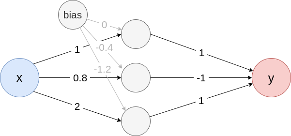
Fig. 1: Example neural network

Create the model from Fig. 1

model <- list(
  input_dim = 1,
  input_nodes = 1,
  input_names = c("x"),
  output_nodes = 2,
  output_names = c("y"),
  layers = list(
    list(
      type = "Dense",
      input_layers = 0,
      output_layers = 2,
      weight = matrix(c(1, 0.8, 2), nrow = 3),
      bias = c(0, -0.4, -1.2),
      activation_name = "relu"
    ),
    list(
      type = "Dense",
      input_layers = 1,
      output_layers = -1,
      weight = matrix(c(1, -1, 1), nrow = 1),
      bias = c(0),
      activation_name = "tanh"
    )
  )
)

converter <- convert(model)

Vanilla Gradient

One of the first and most intuitive methods for interpreting neural networks is the Gradients method introduced by Simonyan et al. (2013), also known as Vanilla Gradients or Saliency maps. This method computes the gradients of the selected output with respect to the input variables. Therefore the resulting relevance values indicate prediction-sensitive variables, i.e., those variables that can be locally perturbed the least to change the outcome the most. Mathematically, this method can be described by the following formula for the input variable $x_i$ with $x \in \mathbb{R}^n$, the model $f:\mathbb{R}^n \to \mathbb{R}^C$ and the output $y_c = f(x)_c$ of class $c$: $$\text{Gradient}(x)_i^c = \frac{\partial\ f(x)_c}{\partial\ x_i} = \frac{\partial\ y_c}{\partial\ x_i}$$

As described in the introduction of this section, the corresponding innsight-method Gradient inherits from the super class InterpretingMethod, meaning that we need to change the term Method to Gradient. Alternatively, an object of the class Gradient can also be created using the mentioned helper function run_grad(), which does not require prior knowledge of R6 objects. The only model-specific argument is times_input, which can be used to switch between the two methods Gradient (default FALSE) and Gradient$\times$Input (TRUE). For more information on the method Gradient$\times$Input see this subsection.

# R6 class syntax
grad <- Gradient$new(converter, data,
  times_input = FALSE,
  ... # other arguments inherited from 'InterpretingMethod'
)

# Using the helper function 
grad <- run_grad(converter, data,
  times_input = FALSE,
  ... # other arguments inherited from 'InterpretingMethod'
)

Example with visualization

In this example, we want to describe the data point $x_1 = 0.45$ with the Gradient method. In principle, the slope of the tangent in $x_1$ is calculated and thus the local rate of change, which in this case is $\tanh'(x_1) = \frac{1}{\cosh(x_1)^2} = 0.822$ (see the red line in Fig. 2). Assuming that the function behaves linearly overall, increasing $x$ by one raises the output by $0.822$. In general, however, neural networks are highly nonlinear, so this interpretation is only valid for very small changes of $x_1$ as you can see in Fig. 2.

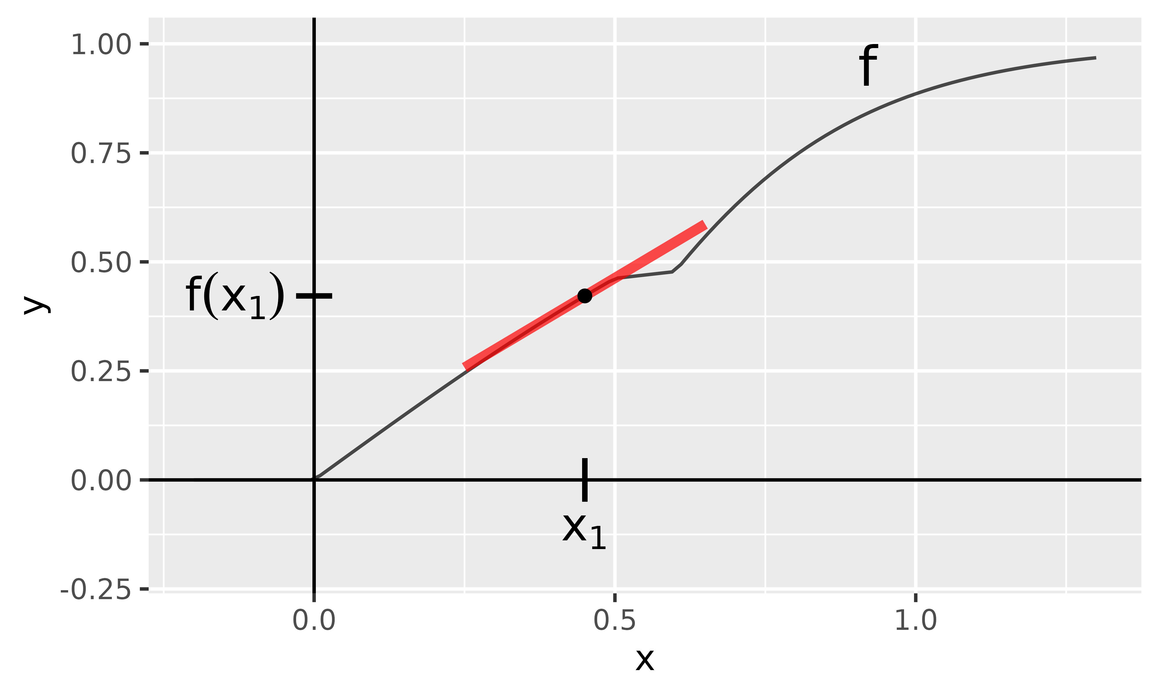
Fig. 2: Gradient method

With innsight, this method is applied as follows and we receive the same result:

data <- matrix(c(0.45), 1, 1)

# Apply method (but don't ignore last activation)
grad <- run_grad(converter, data, ignore_last_act = FALSE)
# get result
get_result(grad)
#> , , y
#> 
#>              x
#> [1,] 0.8220012

SmoothGrad

The SmoothGrad method, introduced by Smilkov et al. (2017), addresses a significant problem of the basic Gradient method. As described in the previous subsection, gradients locally assume a linear behavior, but this is generally no longer the case for deep neural networks. These have large fluctuations and abruptly change their gradients, making the interpretations of the gradient worse and potentially misleading. Smilkov et al. proposed that instead of calculating only the gradient in $x$, compute the gradients of randomly perturbed copies of $x$ and determine the mean gradient from that. To use the SmoothGrad method to obtain relevance values for the individual components $x_i \in \mathbb{R}$ of an instance $x \in \mathbb{R^n}$, we first generate $K \in \mathbb{N}$ realizations of a multivariate Gaussian distribution $p = \mathcal{N}(0, \sigma^2)$ describing the random perturbations, i.e., $\varepsilon^1, \ldots, \varepsilon^K \sim p$. Then the empirical mean of the gradients for variable $x_i$ and output index $c$ can be calculated as follows:

$$\text{SmoothGrad}(x)_i^c = \frac{1}{K} \sum_{j = 1}^K \frac{\partial\ f(x + \varepsilon^j)_c}{\partial\ x_i + \varepsilon_i^j} \approx \mathbb{E}_{\varepsilon \sim p}\left[ \frac{\partial\ f(x + \varepsilon)_c}{\partial\ x_i + \varepsilon_i^j}\right]$$

As described in the introduction of this section, the innsight method SmoothGrad inherits from the super class InterpretingMethod, meaning that we need to change the term Method to SmoothGrad or use the helper function run_smoothgrad() for initializing an object of class SmoothGrad. In addition, there are the following three model-specific arguments:

• n (default: 50): This integer value specifies how many perturbations will be used to calculate the mean gradient, i.e., the $K$ from the formula above. However, it must be noted that the computational effort increases by a factor of n compared to the Gradient method since the simple Gradient method is used n times instead of once. In return, the accuracy of the estimator increases with a larger n.

• noise_level (default: 0.1): With this argument, the strength of the spread of the Gaussian distribution can be given as a percentage, i.e., noise_level $=\frac{\sigma}{\max(x)-\min(x)}$.

• times_input (default: FALSE): Similar to the Gradient method, this argument can be used to switch between the two methods SmoothGrad (FALSE) and SmoothGrad$\times$Input (TRUE). For more information on the method SmoothGrad$\times$Input see this subsection.

# R6 class syntax
smoothgrad <- SmoothGrad$new(converter, data,
  n = 50,
  noise_level = 0.1,
  times_input = FALSE,
  ... # other arguments inherited from 'InterpretingMethod'
)

# Using the helper function 
smoothgrad <- run_smoothgrad(converter, data,
  n = 50,
  noise_level = 0.1,
  times_input = FALSE,
  ... # other arguments inherited from 'InterpretingMethod'
)

Example with visualization

We want to describe the data point $x_1 = 0.6$ with the method SmoothGrad. As you can see in Figure 3, this point does not have a unique gradient because it is something around $0.15$ from the left and something around $1.66$ from the right. In such situations, SmoothGrad comes in handy. As described before, the input $x_1$ is slightly perturbed by a Gaussian distribution and then the mean gradient is calculated. The individual gradients of the perturbed copies are visualized in blue in Figure 3 with the red line representing the mean gradient.

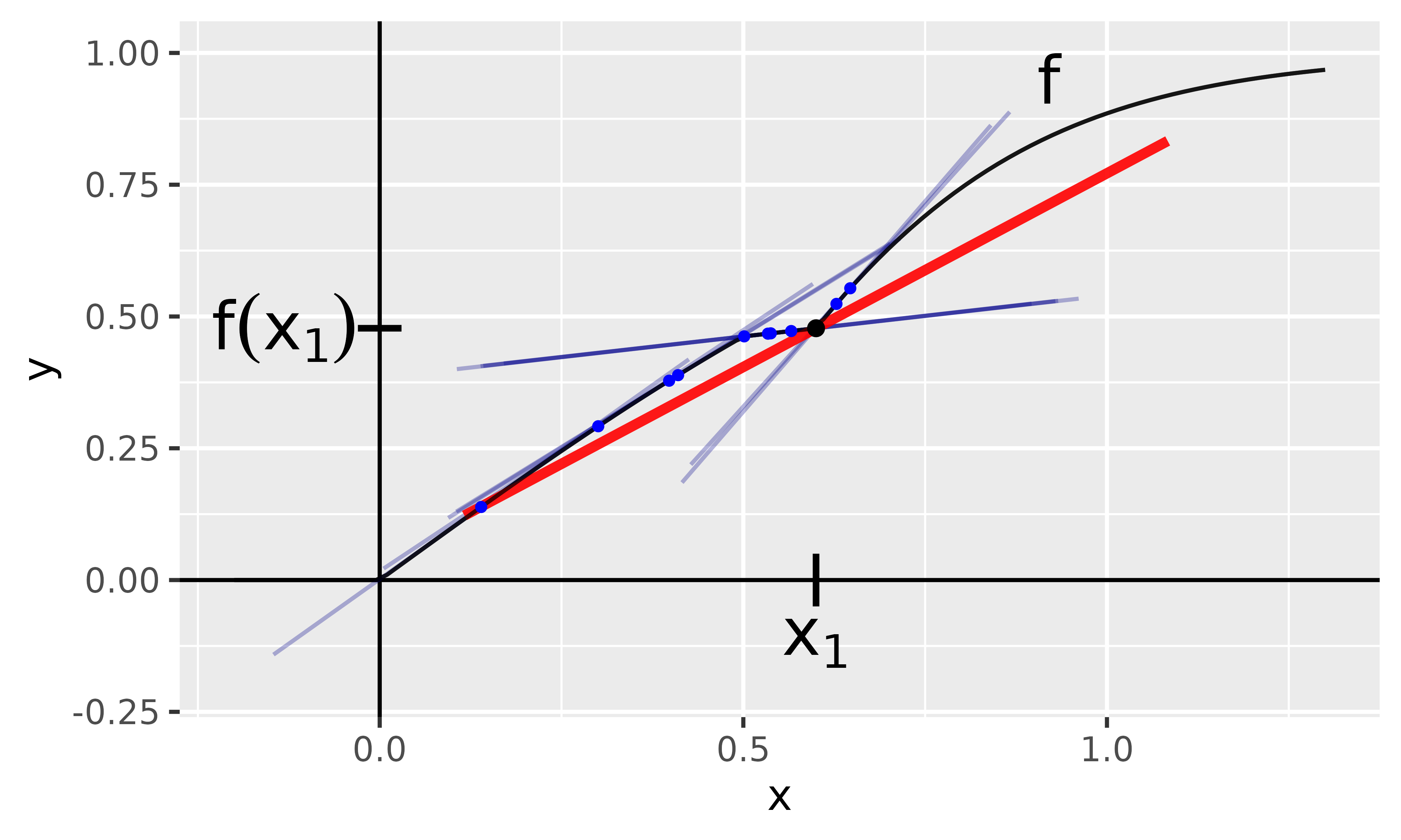
Fig. 3: SmoothGrad method

With innsight, this method is applied as follows:

data <- matrix(c(0.6), 1, 1)

# Apply method
smoothgrad <- run_smoothgrad(converter, data,
  noise_level = 0.2,
  n = 50,
  ignore_last_act = FALSE # include the tanh activation
) 
# get result
get_result(smoothgrad)
#> , , y
#> 
#>              x
#> [1,] 0.8371726

Gradient$\times$Input and SmoothGrad$\times$Input

The methods Gradient$\times$Input and SmoothGrad$\times$Input are as simple as they sound: the gradients are calculated as in the gradient section and then multiplied by the respective input. They were introduced by Shrikumar et al. (2016) and have a well-grounded mathematical background despite their simple idea. The basic idea is to decompose the output according to its relevance to each input variable, i.e., we get variable-wise additive effects

$$\tag{1} f(x)_c = \sum_{i = 1}^n R_i.$$

Mathematically, this method is based on the first-order Taylor decomposition. Assuming that the function $f$ is continuously differentiable in $x \in \mathbb{R}^n$, a remainder term $\varepsilon(f,z,x):\mathbb{R}^n \to \mathbb{R}$ with $\lim_{z \to x} \varepsilon(f, z, x) = 0$ exists such that

$$\begin{align} f(z) &= f(x) + \nabla_x\ f(x)(z-x)^T + \varepsilon(f, z, x)\\ &= f(x) + \sum_{i = 1}^n \frac{\partial\ f(x)}{\partial\ x_i} (z_i - x_i) + \varepsilon(f, z, x), \quad z\in \mathbb{R}^n. \tag{2} \end{align}$$ The first-order Taylor formula thus describes a linear approximation of the function $f$ at the point $x$ since only the first derivatives are considered. Consequently, a highly nonlinear function $f$ is well approximated in a small neighborhood around $x$. For larger distances from $x$, sufficient small values of the residual term are not guaranteed anymore. The Gradient$\times$Input method now considers the data point $x$ and sets $z = 0$. In addition, the residual term and the summand $f(0)_c$ are ignored, which then results in the following approximation of $f(x)_c$ in variable-wise relevances

$$ f(x)_c \approx \sum_{i = 1}^n \frac{\partial\ f(x)_c}{\partial\ x_i} \cdot x_i, \quad \text{hence}\\ \text{Gradient$\times$Input}(x)_i^c = \frac{\partial\ f(x)_c}{\partial\ x_i} \cdot x_i. $$

Derivation from Eq. 2

$$\begin{align} &f(z)_c = f(x)_c + \sum_{i = 1}^n \frac{\partial\ f(x)_c}{\partial\ x_i} (z_i - x_i) + \varepsilon(f, z, x)\\ \Leftrightarrow\quad & f(x)_c = f(z)_c - \sum_{i = 1}^n \frac{\partial\ f(x)_c}{\partial\ x_i} (z_i - x_i) - \varepsilon(f, z, x)\\ \Leftrightarrow\quad & f(x)_c = f(z)_c + \sum_{i = 1}^n \frac{\partial\ f(x)_c}{\partial\ x_i} (x_i - z_i) - \varepsilon(f, z, x) \end{align}$$ Hence, we get for $z = 0$ and after ignoring the remainder term and the value $f(0)_c$$$\begin{align} f(x)_c &= f(0)_c + \sum_{i = 1}^n \frac{\partial\ f(x)_c}{\partial\ x_i} x_i - \varepsilon(f, z, x) \tag{3}\\ &\approx \sum_{i = 1}^n \frac{\partial\ f(x)_c}{\partial\ x_i} x_i \end{align}$$

Analogously, this multiplication is also applied to the SmoothGrad method in order to compensate for local fluctuations: $$\text{SmoothGrad$\times$Input}(x)_i^c = \frac{1}{K} \sum_{j = 1}^K \frac{\partial\ f(x + \varepsilon^j)_c}{\partial\ x_i + \varepsilon_i^j} \cdot (x_i + \varepsilon_i^j),\quad \varepsilon^1, \ldots, \varepsilon^K \sim \mathcal{N}(0,\sigma^2).$$

Both methods are variants of the respective gradient methods Gradient and SmoothGrad and also have the corresponding model-specific arguments and helper functions for the initialization. These variants can be chosen with the argument times_input:

# the "x Input" variant of method "Gradient"
grad_x_input <- Gradient$new(converter, data,
  times_input = TRUE,
  ... # other arguments of method "Gradient"
) 

# the same using the corresponding helper function
grad_x_input <- run_grad(converter, data,
  times_input = TRUE,
  ... # other arguments of method "Gradient"
) 

# the "x Input" variant of method "SmoothGrad"
smoothgrad_x_input <- SmoothGrad$new(converter, data,
  times_input = TRUE,
  ... # other arguments of method "SmoothGrad"
)

# the same using the corresponding helper function
smoothgrad_x_input <- run_smoothgrad(converter, data,
  times_input = TRUE,
  ... # other arguments of method "SmoothGrad"
)

Example with visualization

Gradient$\times$Input:

Now let us describe the data point $x_1 = 0.49$ using the model defined in this chapter’s introduction. For this model holds the equation $f(0) = 0$; therefore, the approximation error is only the negative value of the remainder term at $0$ (as seen in Eq. 3). In Figure 4, the Taylor approximation is drawn in red and at position $0$, you can also see the value of the remainder term (because all other summands are zero). At the same time, the red dot describes the result of the Gradient$\times$Input method, which indeed deviates from the actual value only by the negative of the remainder term at position $0$.

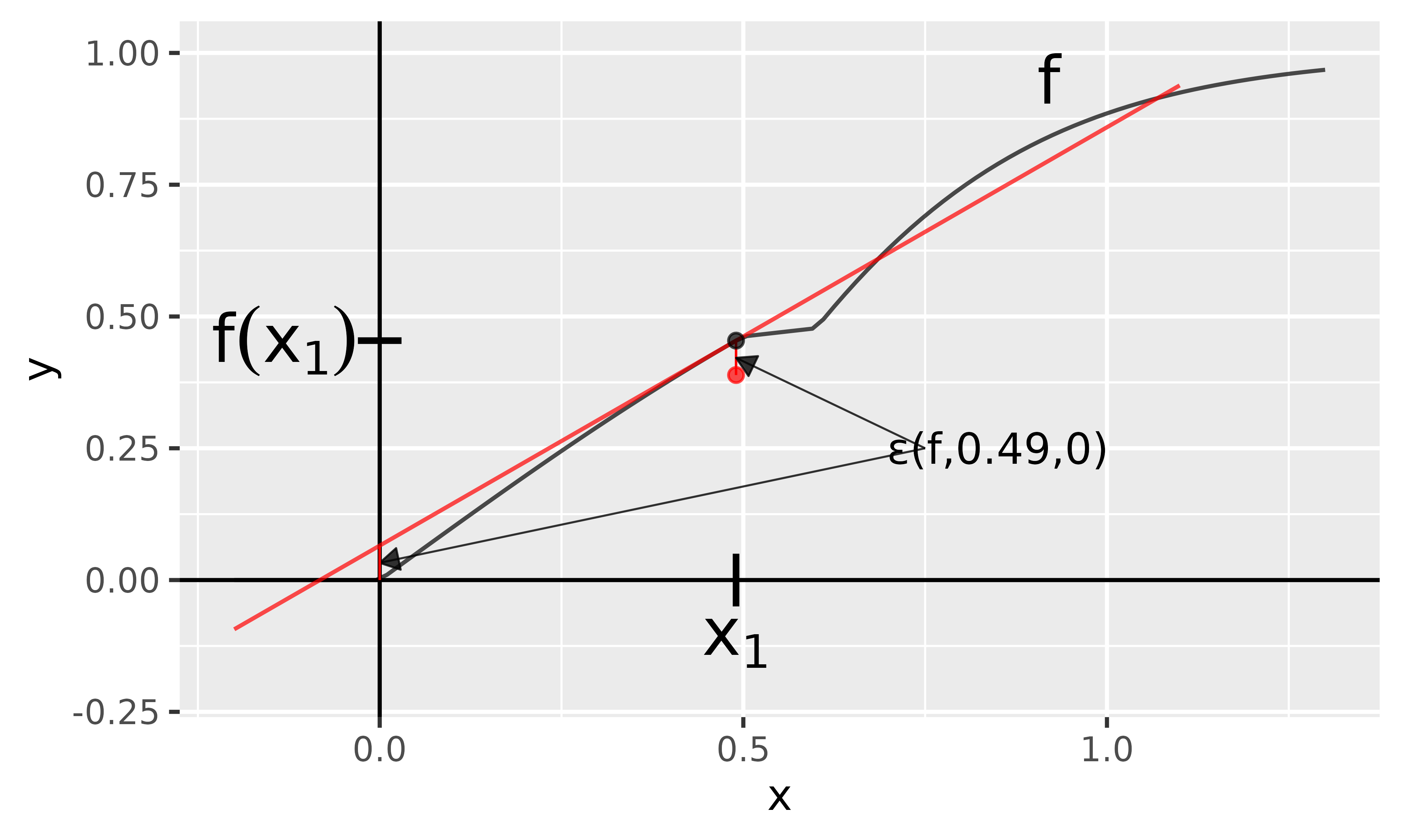
Fig. 4: Gradient$\times$Input method

With innsight, this method is applied as follows:

data <- matrix(c(0.49), 1, 1)

# Apply method
grad_x_input <- run_grad(converter, data,
  times_input = TRUE,
  ignore_last_act = FALSE # include the tanh activation
) 
# get result
get_result(grad_x_input)
#> , , y
#> 
#>              x
#> [1,] 0.3889068

SmoothGrad$\times$Input:

It is also possible to use the SmoothGrad$\times$Input method to perturb the input $x_1 = 0.49$ a bit and return an average value of the individual Gradient$\times$Input results. Figure 5 shows the individual linear approximations of the first-order Taylors for the Gaussian perturbed copies of $x_1$, and the blue dots describe the respective Gradient$\times$Input values. The red dot represents the mean value, i.e., the value of the SmoothGrad$\times$Input method at $x_1 = 0.49$.

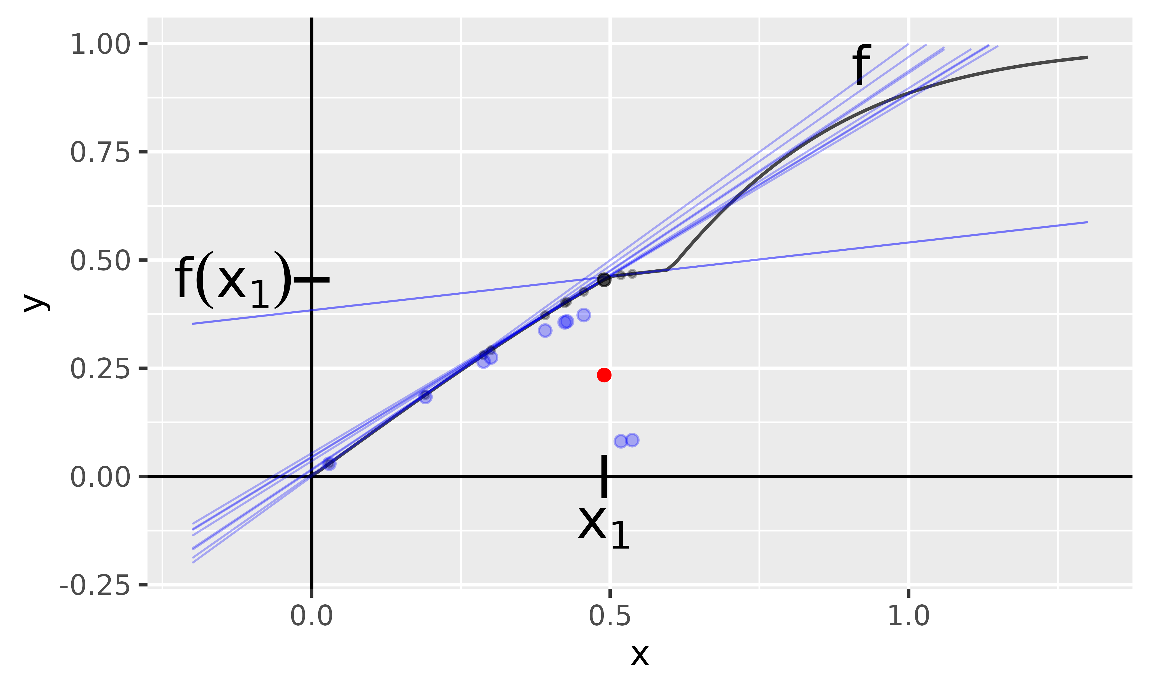
Fig. 5: SmoothGrad$\times$Input method

With innsight, this method is applied as follows:

data <- matrix(c(0.49), 1, 1)

# Apply method
smoothgrad_x_input <- run_smoothgrad(converter, data,
  times_input = TRUE,
  ignore_last_act = FALSE # include the tanh activation
) 
# get result
get_result(smoothgrad_x_input)
#> , , y
#> 
#>              x
#> [1,] 0.3008178

Layer-wise Relevance Propagation (LRP)

The LRP method was first introduced by Bach et al. (2015) and has a similar goal to the Gradient$\times$Input approach explained in the last section: decompose the output into variable-wise relevances according to Eq. 1. The difference is that the prediction $f(x)_c = y_c$ is redistributed layer by layer from the output node back to the inputs according to the weights and pre-activations. This is done by so-called relevance messages $r_{i \leftarrow j}^{(l, l+1)}$, which can be defined by a rule on redistributing the upper-layer relevance $R_j^{l +1}$ to the lower-layer $R_i^{l}$. In the package innsight, the following commonly used rules are defined ($i$ is an index of a node in layer $l$ and $j$ an index of a node in layer $l+1$):

• The simple rule (also known as LRP-0)
  This is the most basic rule on which all other rules are more or less based. The relevances are redistributed to the lower layers according to the ratio between local and global pre-activation. Let $x_i$ the inputs, $w_{i,j}$ the weights and $b_j$ the bias vector of layer $l$ and $R_j^{(l+1)}$ the upper-layer relevance, then the simple rule is defined as $$r_{i \leftarrow j}^{(l, l+1)} = \frac{x_i\, w_{i,j}}{z_j} \, R_j^{l +1} \quad \text{with} \quad z_j = b_j + \sum_{k} x_k\, w_{k,j}.$$

• The $\varepsilon$-rule (also known as LRP-$\epsilon$)
  One problem with the simple rule is that it is numerically unstable when the global pre-activation $z_j$ vanishes and causes a division by zero. This problem is solved in the $\varepsilon$-rule by adding a stabilizer $\varepsilon > 0$ that moves the denominator away from zero, i.e., $$r_{i \leftarrow j}^{(l, l+1)} = \frac{x_i\, w_{i,j}}{z_j + \text{sign}(z_j)\, \varepsilon}\, R_j^{l +1}.$$

• The $\alpha$-$\beta$-rule (also known as LRP-$\alpha \beta$)
  Another way to avoid this numerical instability is by treating the positive and negative pre-activations separately. In this case, positive and negative values cannot cancel each other out, i.e., a vanishing denominator also results in a vanishing numerator. Moreover, this rule allows choosing a weighting for the positive and negative relevances, which is done with the parameters $\alpha, \beta \in \mathbb{R}$ satisfying $\alpha + \beta = 1$. The $\alpha$-$\beta$-rule is defined as $$ r_{i \leftarrow j}^{(l, l+1)} = \left(\alpha \frac{(x_i\, w_{i,j})^+}{z_j^+} + \beta \frac{(x_i\, w_{i,j})^-}{z_j^-}\right)\, R_j^{l +1}\\ \text{with}\quad z_j^\pm = (b_j)^\pm + \sum_k (x_k\, w_{k,j})^\pm,\quad (\cdot)^+ = \max(\cdot, 0),\quad (\cdot)^- = \min(\cdot, 0). $$

For any of the rules described above, the relevance of the lower-layer nodes $R_i^{l}$ is determined by summing up all incoming relevance messages $r_{i \leftarrow j}^{(l, l +1)}$ into the respective node of index $i$, i.e., $$R_i^{l} = \sum_j r_{i \leftarrow j}^{(l, l +1)}.$$

This procedure is repeated layer by layer until one gets to the input layer and consequently gets the relevances for each input variable. A visual overview of the entire method using the simple rule as an example is given in Fig. 6.

📝 Note
At this point, it must be mentioned that the LRP variants do not lead to an exact decomposition of the output since some of the relevance is absorbed by the bias terms. This is because the bias is included in the pre-activation but does not appear in any of the numerators.

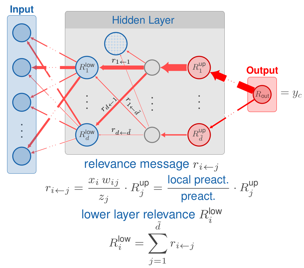
Fig. 6: Layerwise Relevance Propagation

Analogous to the previous methods, the innsight method LRP inherits from the InterpretingMetod super class and thus all arguments. In addition, there are the following method-specific arguments for this method:

• rule_name (default: "simple"): This argument can be used to select the rule for the relevance messages. Implemented are the three rules described above, i.e., simple rule ("simple"), $\varepsilon$-rule ("epsilon") and $\alpha$-$\beta$-rule ("alpha_beta"). However, a named list can also be passed to assign one of these three rules to each implemented layer type individually. Layers not specified in this list then use the default value "simple". For example, with list(Dense_Layer = "epsilon", Conv2D_Layer = "alpha_beta") the simple rule is used for all dense layers and the $\alpha$-$\beta$-rule is applied to all 2D convolutional layers. The other layers not mentioned use the default rule. In addition, for normalization layers like 'BatchNorm_Layer', the rule "pass" is implemented as well, which ignores such layers in the backward pass. You can set the rule for the following layer types:

  • 'Dense_Layer', 'Conv1D_Layer', 'Conv2D_Layer', 'BatchNorm_Layer', 'AvgPool1D_Layer', 'AvgPool2D_Layer', 'MaxPool1D_Layer' and 'MaxPool2D_Layer'

• rule_param: The meaning of this argument depends on the selected rule. For the simple rule, for example, it has no effect. In contrast, this numeric argument sets the value of $\varepsilon$ for the $\varepsilon$-rule and the value of $\alpha$ for the $\alpha$-$\beta$-rule (remember: $\beta = 1 - \alpha$). Passing NULL defaults to 0.01 for $\varepsilon$ or 0.5 for $\alpha$. Similar to the argument rule_name, this can also be a named list that individually assigns a rule parameter to each layer type.

• winner_takes_all: This logical argument is only relevant for models with a MaxPooling layer. Since many zeros are produced during the backward pass due to the selection of the maximum value in the pooling kernel, another variant is implemented, which treats a MaxPooling as an AveragePooling layer in the backward pass to overcome the problem of too many zero relevances. With the default value TRUE, the whole upper-layer relevance is passed to the maximum value in each pooling window. Otherwise, if FALSE, the relevance is distributed equally among all nodes in a pooling window.

# R6 class syntax
lrp <- LRP$new(converter, data,
  rule_name = "simple",
  rule_param = NULL,
  winner_takes_all = TRUE,
  ... # other arguments inherited from 'InterpretingMethod'
) 

# Using the helper function for initialization
lrp <- run_lrp(converter, data,
  rule_name = "simple",
  rule_param = NULL,
  winner_takes_all = TRUE,
  ... # other arguments inherited from 'InterpretingMethod'
) 

Example

First, let’s look again at the result at the point $x_1 = 0.49$, which was about $0.3889$ when approximated with the Gradient$\times$Input method. For LRP with the simple rule, we get $0.4542$ which exactly matches the actual value of $f(x_1)$. This is mainly due to the fact that for an input of $x_1$, only the top neuron from Fig. 1 is activated and it does not have a bias term. However, if we now use an input that activates a neuron with a bias term ($x_2 = 0.6$), there will be an approximation error (for $x_2$ it’s $-0.3675$) since it absorbs some of the relevance. See the code below:

# We can analyze multiple inputs simultaneously
data <- matrix(
  c(
    0.49, # only neuron without bias term is activated
    0.6   # neuron with bias term is activated
  ), 
  ncol = 1
)

# Apply LRP with simple rule
lrp <- run_lrp(converter, data,
  ignore_last_act = FALSE
)
get_result(lrp)
#> , , y
#> 
#>              x
#> [1,] 0.4542146
#> [2,] 0.1102428

# get approximation error
matrix(lrp$get_result()) - as_array(converter$model(torch_tensor(data))[[1]])
#>               [,1]
#> [1,] -1.877546e-06
#> [2,] -3.674572e-01

The individual LRP variants can also be considered as a function in the input variable $x$, which is shown in Fig. 7 with the true model $f$ in black.

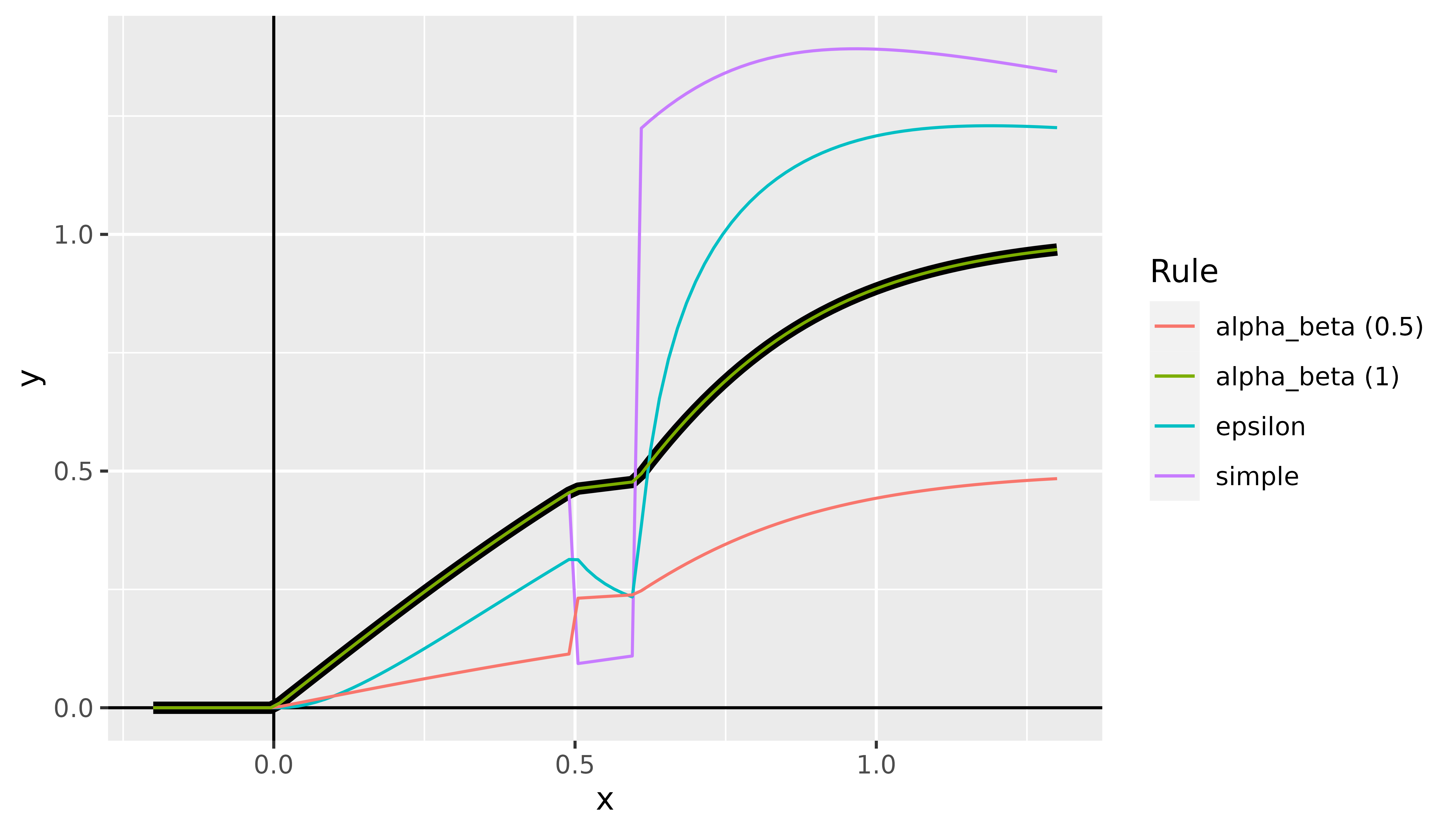
Fig. 7: LRP method

Deep Learning Important Features (DeepLift)

One method that, to some extent, echoes the idea of LRP is the so-called Deep Learning Important Features (DeepLift) method introduced by Shrikumar et al. in 2017. It behaves similarly to LRP in a layer-by-layer backpropagation fashion from a selected output node back to the input variables. However, it incorporates a reference value $\tilde{x}$ to compare the relevances with each other. Hence, the relevances of DeepLift represent the relative effect of the outputs of the instance to be explained $f(x)_c$ and the output of the reference value $f(\tilde{x})_c$, i.e., $f(x)_c - f(\tilde{x})_c$. This difference eliminates the bias term in the relevance messages so that no more relevance is absorbed and we have an exact variable-wise decomposition of $\Delta y = f(x)_c - f(\tilde{x})_c$. In addition, the authors presented two rules to propagate relevances through the activation part of the individual layers, namely Rescale and RevealCancel rule. The Rescale rule simply scales the contribution to the difference from reference output according to the value of the activation function. The RevealCancel rule considers the average impact after adding the negative or positive contribution revealing dependencies missed by other approaches.

Analogous to the previous methods, the innsight method DeepLift inherits from the InterpretingMetod super class and thus all arguments. Alternatively, an object of the class DeepLift can also be created using the helper function run_deeplift(), which does not require prior knowledge of R6 objects. In addition, there are the following method-specific arguments for this method:

• x_ref (default: NULL): This argument describes the reference input $\tilde{x}$ for the DeepLift method. This value must have the same format as the input data of the passed model to the converter class, i.e.,

  • an array, data.frame, torch_tensor or array-like format of size $\left(1, \text{input_dim}\right)$ or
  • a list with the corresponding input data (according to the upper point) for each of the input layers.
  • It is also possible to use the default value NULL to take only zeros as reference input.

• rule_name (default: 'rescale'): Name of the applied rule to calculate the contributions. Use either 'rescale' or 'reveal_cancel'.

• winner_takes_all: This logical argument is only relevant for MaxPooling layers and is otherwise ignored. With this layer type, it is possible that the position of the maximum values in the pooling kernel of the normal input $x$ and the reference input $\tilde{x}$ may not match, which leads to a violation of the summation-to-delta property. To overcome this problem, another variant is implemented, which treats a MaxPooling layer as an AveragePooling layer in the backward pass only, leading to a uniform distribution of the upper-layer contribution to the lower layer.

# R6 class syntax
deeplift <- DeepLift$new(converter, data,
  x_ref = NULL,
  rule_name = "rescale",
  winner_takes_all = TRUE,
  ... # other arguments inherited from 'InterpretingMethod'
) 

# Using the helper function for initialization
deeplift <- run_deeplift(converter, data,
  x_ref = NULL,
  rule_name = "rescale",
  winner_takes_all = TRUE,
  ... # other arguments inherited from 'InterpretingMethod'
) 

Examples

In this example, let’s consider the point $x = 0.55$ and the reference point $\tilde{x} = 0.1$. With the help of the model defined previously, the respective outputs are $y = f(x) = 0.4699$ and $\tilde{y} = f(\tilde{x}) = 0.0997$. The DeepLift method now generates an exact variable-wise decomposition of the so-called difference-from-reference value $\Delta y = y - \tilde{y} = 0.3702772$. Since there is only one input feature in this case, the entire value should be assigned to it:

# Create data
x <- matrix(c(0.55))
x_ref <- matrix(c(0.1))

# Apply method DeepLift with rescale rule
deeplift <- run_deeplift(converter, x, x_ref = x_ref, ignore_last_act = FALSE)

# Get result
get_result(deeplift)
#> , , y
#> 
#>              x
#> [1,] 0.3702772

This example is an extremely simple model, so we will test this method on a slightly larger model and the Iris dataset (see ?iris):

library(neuralnet)
set.seed(42)

# Crate model with package 'neuralnet'
model <- neuralnet(Species ~ ., iris, hidden = 5, linear.output = FALSE)

# Step 1: Create 'Converter'
conv <- convert(model)

# Step 2: Apply DeepLift (reveal-cancel rule)
x_ref <- matrix(colMeans(iris[, -5]), nrow = 1) # use colmeans as reference value
deeplift <- run_deeplift(conv, iris[, -5],
  x_ref = x_ref, ignore_last_act = FALSE,
  rule_name = "reveal_cancel"
)

# Verify exact decomposition
y <- predict(model, iris[, -5])
y_ref <- predict(model, x_ref[rep(1, 150), ])
delta_y <- y - y_ref
summed_decomposition <- apply(get_result(deeplift), c(1, 3), FUN = sum) # dim 2 is the input feature dim

# Show the mean squared error
mean((delta_y - summed_decomposition)^2)
#> [1] 1.603259e-14

Integrated Gradients

In the Integrated Gradients method introduced by Sundararajan et al. (2017), the gradients are integrated along a path from the value $x$ to a reference value $\tilde{x}$. This integration results, similar to DeepLift, in a decomposition of $f(x) - f(\tilde{x})$. In this sense, the method uncovers the feature-wise relative effect of the input features on the difference between the prediction $f(x)$ and the reference prediction $f(\tilde{x})$. This is archived through the following formula: $$\text{IntGrad}(x)_i^c = (x - \tilde{x}) \int_{\alpha = 0}^1 \frac{\partial f(\tilde{x} + \alpha (x - \tilde{x}))}{\partial x} d\alpha$$ In simpler terms, it calculates how much each feature contributes to a model’s output by tracing a path from a baseline input $\tilde{x}$ to the actual input $x$ and measuring the average gradients along that path.

Similar to the other gradient-based methods, by default the integrated gradient is multiplied by the input to get an approximate decomposition of $f(x) - f(\tilde{x})$. However, with the parameter times_input only the gradient describing the output sensitivity can be returned.

Analogous to the previous methods, the innsight method IntegratedGradient inherits from the InterpretingMetod super class and thus all arguments. Alternatively, an object of the class IntegratedGradient can also be created using the helper function run_intgrad(), which does not require prior knowledge of R6 objects. In addition, there are the following method-specific arguments for this method:

• x_ref (default: NULL): This argument describes the reference input $\tilde{x}$ for the Integrated Gradients method. This value must have the same format as the input data of the passed model to the converter class, i.e.,

  • an array, data.frame, torch_tensor or array-like format of size $\left(1, \text{input_dim}\right)$ or
  • a list with the corresponding input data (according to the upper point) for each of the input layers.
  • It is also possible to use the default value NULL to take only zeros as reference input.

• n (default: 50): Number of steps for the approximation of the integration path along $\alpha$.

• times_input (default: TRUE): Multiplies the integrated gradients with the difference of the input features and the baseline values. By default, the original definition of Integrated Gradient is applied. However, by setting times_input = FALSE only an approximation of the integral is calculated, which describes the sensitivity of the features to the output.

# R6 class syntax
intgrad <- IntegratedGradient$new(converter, data,
  x_ref = NULL,
  n = 50,
  times_input = TRUE,
  ... # other arguments inherited from 'InterpretingMethod'
) 

# Using the helper function for initialization
intgrad <- run_intgrad(converter, data,
  x_ref = NULL,
  n = 50,
  times_input = TRUE,
  ... # other arguments inherited from 'InterpretingMethod'
) 

Examples

In this example, let’s consider the point $x = 0.55$ and the reference point $\tilde{x} = 0.1$. With the help of the model defined previously, the respective outputs are $y = f(x) = 0.4699$ and $\tilde{y} = f(\tilde{x}) = 0.0997$. The Integrated Gradient method now generates an approximate variable-wise decomposition of the so-called difference-from-reference value $\Delta y = y - \tilde{y} = 0.3702772$. Since there is only one input feature in this case, the entire value should be assigned to it:

# Create data
x <- matrix(c(0.55))
x_ref <- matrix(c(0.1))

# Apply method IntegratedGradient
intgrad <- run_intgrad(converter, x, x_ref = x_ref, ignore_last_act = FALSE)

# Get result
get_result(intgrad)
#> , , y
#> 
#>              x
#> [1,] 0.3668411

Expected Gradients

The Expected Gradients method (Erion et al., 2021), also known as GradSHAP, is a local feature attribution technique which extends the Integrated Gradient method and provides approximate Shapley values. In contrast to Integrated Gradient, it considers not only a single reference value $\tilde{x}$ but the whole distribution of reference values $\tilde{X} \sim \tilde{x}$ and averages the Integrated Gradient values over this distribution. Mathematically, the method can be described as follows: $$\text{ExpGrad}(x)_i^c = \mathbb{E}_{\tilde{x}\sim \tilde{X}, \alpha \sim U(0,1)} \left[(x - \tilde{x}) \times \frac{\partial f(\tilde{x} + \alpha (x - \tilde{x}))}{\partial x} \right]$$ These feature-wise values approximate a decomposition of the prediction minus the average prediction in the reference dataset, i.e., $f(x) - \mathbb{E}_{\tilde{x}}\left[f(\tilde{x}) \right]$. This means, it solves the issue of choosing the right reference value.

Analogous to the previous methods, the innsight method ExpectedGradient inherits from the InterpretingMetod super class and thus all arguments. Alternatively, an object of the class ExpectedGradient can also be created using the helper function run_expgrad(), which does not require prior knowledge of R6 objects. In addition, there are the following method-specific arguments for this method:

• data_ref (default: NULL): This argument describes the reference inputs $\tilde{x}$ for the Expected Gradients method. This value must have the same format as the input data of the passed model to the converter class, i.e.,

  • an array, data.frame, torch_tensor or array-like format of size $\left(1, \text{input_dim}\right)$ or
  • a list with the corresponding input data (according to the upper point) for each of the input layers.
  • It is also possible to use the default value NULL to take only zeros as reference input.

• n (default: 50): Number of samples from the distribution of reference values $\tilde{x} \sim \tilde{X}$ and number of samples for the approximation of the integration path along $\alpha$.

# R6 class syntax
expgrad <- ExpectedGradient$new(converter, data,
  data_ref = NULL,
  n = 50,
  ... # other arguments inherited from 'InterpretingMethod'
) 

# Using the helper function for initialization
expgrad <- run_expgrad(converter, data,
  x_ref = NULL,
  n = 50,
  ... # other arguments inherited from 'InterpretingMethod'
) 

Examples

In the following example, we demonstrate how the Expected Gradient method is applied to the Iris dataset, accurately approximating the difference between the prediction and the mean prediction (adjusted for a very high sample size of $10\,000$):

library(neuralnet)
set.seed(42)

# Crate model with package 'neuralnet'
model <- neuralnet(Species ~ ., iris, linear.output = FALSE)

# Step 1: Create 'Converter'
conv <- convert(model)

# Step 2: Apply Expected Gradient
expgrad <- run_expgrad(conv, iris[c(1, 60), -5],
  data_ref = iris[, -5], ignore_last_act = FALSE,
  n = 10000
)

# Verify exact decomposition
y <- predict(model, iris[, -5])
delta_y <- y[c(1, 60), ] - rbind(colMeans(y), colMeans(y))
summed_decomposition <- apply(get_result(expgrad), c(1, 3), FUN = sum) # dim 2 is the input feature dim

# Show the error between both
delta_y - summed_decomposition
#>           setosa   versicolor    virginica
#> [1,] -0.09275329 -0.003985501 -0.001253287
#> [2,]  0.01313814  0.001135939 -0.003019490

DeepSHAP

The DeepSHAP method (Lundberg & Lee, 2017) extends the DeepLift technique by not only considering a single reference value but by calculating the average from several, ideally representative reference values at each layer. The obtained feature-wise results are approximate Shapley values for the chosen output, where the conditional expectation is computed using these different reference values, i.e., the DeepSHAP method decompose the difference from the prediction and the mean prediction $f(x) - \mathbb{E}_{\tilde{x}}\left[f(\tilde{x}) \right]$ in feature-wise effects. This means, the DeepSHAP method has the same underlying goal as the Expected Gradient method and, hence, also solves the issue of choosing the right reference value for the DeepLift method.

Analogous to the previous methods, the innsight method DeepSHAP inherits from the InterpretingMetod super class and thus all arguments. Alternatively, an object of the class DeepSHAP can also be created using the helper function run_deepshap()`, which does not require prior knowledge of R6 objects. In addition, there are the following method-specific arguments for this method:

• data_ref (default: NULL): The reference data which is used to estimate the conditional expectation. These must have the same format as the input data of the passed model to the converter object. This means either

  • an array, data.frame, torch_tensor or array-like format of size $\left(1, \text{input_dim}\right)$ or
  • a list with the corresponding input data (according to the upper point) for each of the input layers.
  • It is also possible to use the default value NULL to take only zeros as reference input.

• limit_ref (default: 100): This argument limits the number of instances taken from the reference dataset data_ref so that only random limit_ref elements and not the entire dataset are used to estimate the conditional expectation. A too-large number can significantly increase the computation time.

• (other model-specific arguments already explained in the DeepLift method, e.g., rule_name or winner_takes_all).

# R6 class syntax
deepshap <- DeepSHAP$new(converter, data,
  data_ref = NULL,
  limit_ref = 100,
  ... # other arguments inherited from 'DeepLift'
) 

# Using the helper function for initialization
deepshap <- run_deepshap(converter, data,
  data_ref = NULL,
  limit_ref = 100,
  ... # other arguments inherited from 'DeepLift'
) 

Examples

In the following example, we demonstrate how the DeepSHAP method is applied to the Iris dataset, accurately approximating the difference between the prediction and the mean prediction (adjusted for a very high sample size of $10\,000$):

library(neuralnet)
set.seed(42)

# Crate model with package 'neuralnet'
model <- neuralnet(Species ~ ., iris, linear.output = FALSE)

# Step 1: Create 'Converter'
conv <- convert(model)

# Step 2: Apply Expected Gradient
deepshap <- run_deepshap(conv, iris[c(1, 60), -5],
  data_ref = iris[, -5], ignore_last_act = FALSE,
  limit_ref = nrow(iris)
)

# Verify exact decomposition
y <- predict(model, iris[, -5])
delta_y <- y[c(1, 60), ] - rbind(colMeans(y), colMeans(y))
summed_decomposition <- apply(get_result(deepshap), c(1, 3), FUN = sum) # dim 2 is the input feature dim

# Show the error between both
delta_y - summed_decomposition
#>             setosa    versicolor   virginica
#> [1,] -1.241763e-09 -6.365796e-09 2.14234e-08
#> [2,] -9.623667e-09 -3.889552e-08 1.62512e-08

Connection Weights

One of the earliest methods specifically for neural networks was the Connection Weights method invented by Olden et al. in 2004, resulting in a global relevance score for each input variable. The basic idea of this approach is to multiply all path weights for each possible connection between an input variable and the output node and then calculate the sum of all of them. However, this method ignores all bias vectors and all activation functions during calculation. Since only the weights are used, this method is independent of input data and, thus, a global interpretation method. In this package, we extended this method to a local one inspired by the method Gradient$\times$Input (see here). Hence, the local variant is simply the point-wise product of the global Connection Weights method and the input data. You can use this variant by setting the times_input argument to TRUE and providing input data.

The innsight method ConnectionWeights also inherits from the super class InterpretingMethod, meaning that you need to change the term Method to ConnectionWeights. Alternatively, an object of the class ConnectionWeights can also be created using the helper function run_cw(), which does not require prior knowledge of R6 objects. The only model-specific argument is times_input, which can be used to switch between the global (FALSE) and the local (TRUE) Connection Weights method.

# The global variant (argument 'data' is no longer required)
cw_global <- ConnectionWeights$new(converter,
  times_input = FALSE,
  ... # other arguments inherited from 'InterpretingMethod'
) 

# The local variant (argument 'data' is required)
cw_local <- ConnectionWeights$new(converter, data,
  times_input = TRUE,
  ... # other arguments inherited from 'InterpretingMethod'
) 

# Using the helper function
cw_local <- run_cw(converter, data,
  times_input = TRUE,
  ... # other arguments inherited from 'InterpretingMethod'
) 

Examples

Since the global Connection Weights method only multiplies the path weights, the result for the input feature $x$ based on Figure 1 is $$(1 \cdot 1) + (0.8 \cdot -1) + (2 \cdot 1) = 2.2.$$ With the innsight package, we get the same value:

# Apply global Connection Weights method
cw_global <- run_cw(converter, times_input = FALSE)

# Show the result
get_result(cw_global)
#> , , y
#> 
#>        x
#> [1,] 2.2

However, the local variant requires input data data and returns instance-wise relevances:

# Create data
data <- array(c(0.1, 0.4, 0.6), dim = c(3, 1))

# Apply local Connection Weights method
cw_local <- run_cw(converter, data, times_input = TRUE)

# Show the result
get_result(cw_local)
#> , , y
#> 
#>              x
#> [1,] 0.2200000
#> [2,] 0.8800001
#> [3,] 1.3200001

Step 3: Show and plot the results

Once a method object has been created, the results can be returned as an array, data.frame, or torch_tensor, and can be further processed as desired. In addition, for each of the three sizes of the inputs (tabular, 1D signals or 2D images) suitable plot and boxplot functions based on ggplot2 are implemented. Due to the complexity of higher dimensional inputs, these plots and boxplots can also be displayed as an interactive plotly plots by using the argument as_plotly. These three class methods have also been implemented as S3 methods (get_result(), plot() and plot_global()/boxplot()) for easier handling.

Create results to be visualized

library(torch)
library(neuralnet)
set.seed(45)

# Model for tabular data
# We use the iris dataset for tabular data
tab_data <- as.matrix(iris[, -5])
tab_data <- t((t(tab_data) - colMeans(tab_data)) / rowMeans((t(tab_data) - colMeans(tab_data))^2))
tab_names <- colnames(tab_data)
out_names <- unique(iris$Species)

tab_model <- neuralnet(Species ~ .,
  data = data.frame(tab_data, Species = iris$Species),
  linear.output = FALSE,
  hidden = 10
)

# Model for image data
img_data <- array(rnorm(5 * 32 * 32 * 3), dim = c(5, 3, 32, 32))

img_model <- nn_sequential(
  nn_conv2d(3, 5, c(3, 3)),
  nn_relu(),
  nn_avg_pool2d(c(2, 2)),
  nn_conv2d(5, 10, c(2, 2)),
  nn_relu(),
  nn_avg_pool2d(c(2, 2)),
  nn_flatten(),
  nn_linear(490, 3),
  nn_softmax(2)
)

# Create converter
tab_conv <- convert(tab_model,
  input_dim = c(4),
  input_names = tab_names,
  output_names = out_names
)

img_conv <- convert(img_model, input_dim = c(3, 32, 32))

# Apply Gradient x Input
tab_grad <- run_grad(tab_conv, tab_data, times_input = TRUE)
img_grad <- run_grad(img_conv, img_data, times_input = TRUE)

Get results

Each instance of the presented interpretability methods has the class method get_result(), which is used to return the results. You can choose between the data formats array, data.frame or torch_tensor by passing the name as a character in the argument type. As mentioned before, there is also a S3 function get_result() for this class method.

# You can use the class method
method$get_result(type = "array")
# or you can use the S3 method
get_result(method, type = "array")

Array (type = 'array')

In the simplest case, when the passed model to the converter object has only one input and one output layer, an R primitive array of dimension $\left(\text{batch_size}, \text{input_dim}, \text{outputs}\right)$ is returned, where $\text{outputs}$ means the number of elements from the argument output_idx. In addition, the passed or generated input and output names are added to the array.

However, this method behaves differently if the passed model has multiple input and/or output layers. In these cases, a list (or a nested list) with the corresponding input and output layers with the associated results is generated as in the simple case from before:

• $n$ input layers and one output layer:

  List of n
    $ Input_1: array [batch_size, input_1_dim, outputs]
    $ Input_2: array [batch_size, input_2_dim, outputs]
    ...
    $ Input_n: array [batch_size, input_n_dim, outputs]

• one input layer and $k$ output layers (outputs_i are the corresponding output indices specified previously in the argument output_idx):

  List of k
    $ Output_1: array [batch_size, input_dim, outputs_1]
    $ Output_2: array [batch_size, input_dim, outputs_2]
    ...
    $ Output_k: array [batch_size, input_dim, outputs_k]

• $n$ input and $k$ output layers (outputs_i are the corresponding output indices specified previously in the argument output_idx):

  List of k
    $ Output_1: List of n
      $ Input_1: array [batch_size, input_1_dim, outputs_1]
      $ Input_2: array [batch_size, input_2_dim, outputs_1]
      ...
      $ Input_n: array [batch_size, input_n_dim, outputs_1]
    $ Output_2: List of n
      $ Input_1: array [batch_size, input_1_dim, outputs_2]
      $ Input_2: array [batch_size, input_2_dim, outputs_2]
      ...
      $ Input_n: array [batch_size, input_n_dim, outputs_2]
    ...
    $ Output_k: List of n
      $ Input_1: array [batch_size, input_1_dim, outputs_k]
      $ Input_2: array [batch_size, input_2_dim, outputs_k]
      ...
      $ Input_n: array [batch_size, input_n_dim, outputs_k]

Example with a tabular model

# Apply method 'Gradient x Input' for classes 1 ('setosa')  and 3 ('virginica')
tab_grad <- run_grad(tab_conv, tab_data,
  output_idx = c(1, 3),
  times_input = TRUE
)
# Get result
result_array <- tab_grad$get_result()
# You can also use the S3 function 'get_result'
result_array <- get_result(tab_grad)

# Show the result for datapoint 1 and 10
result_array[c(1, 10), , ]
#> , , setosa
#> 
#>      Sepal.Length Sepal.Width Petal.Length Petal.Width
#> [1,]   -0.8710907  -0.4592198     3.246672   0.6098831
#> [2,]   -1.1206678  -0.0285231     2.863380   0.6617002
#> 
#> , , virginica
#> 
#>      Sepal.Length Sepal.Width Petal.Length Petal.Width
#> [1,]     1.034490   0.4134942    -2.887100  -0.6511033
#> [2,]     1.406196   0.0178409    -2.672977  -0.7532284

Example with an image model

# Apply method 'Gradient' for outputs 1  and 2
img_grad <- run_grad(img_conv, img_data, output_idx = c(1, 2))
# Get result
result_array <- img_grad$get_result()
# You can also use the S3 function 'get_result'
result_array <- get_result(img_grad)

# Show the result
str(result_array)
#>  num [1:5, 1:3, 1:32, 1:32, 1:2] 8.41e-05 -6.74e-05 1.48e-04 -8.55e-05 -2.91e-05 ...
#>  - attr(*, "dimnames")=List of 5
#>   ..$ : NULL
#>   ..$ : chr [1:3] "C1" "C2" "C3"
#>   ..$ : chr [1:32] "H1" "H2" "H3" "H4" ...
#>   ..$ : chr [1:32] "W1" "W2" "W3" "W4" ...
#>   ..$ : chr [1:2] "Y1" "Y2"

Examples with models with more than one input or output layer

Multiple inputs and one output layer

First, we consider a model with two input layers. In this case, we have a list of the length of the input layers 'Input_1', 'Input_2', … 'Input_n' and each entry contains an named array of shape $\left(\text{batch_size}, \text{input_dim}_i, \text{outputs} \right)$ with $\text{input_dim}_i$ the input shape of input layer 'Input_i':

Create model and data

library(keras)

first_input <- layer_input(shape = c(10, 10, 2))
second_input <- layer_input(shape = c(11))
tmp <- first_input %>%
  layer_conv_2d(2, c(2, 2), activation = "relu") %>%
  layer_flatten() %>%
  layer_dense(units = 11)
output <- layer_add(c(tmp, second_input)) %>%
  layer_dense(units = 5, activation = "relu") %>%
  layer_dense(units = 3, activation = "softmax")
model <- keras_model(
  inputs = c(first_input, second_input),
  outputs = output
)

conv <- convert(model)
#> Skipping InputLayer ...
#> Skipping InputLayer ...
data <- lapply(
  list(c(10, 10, 2), c(11)),
  function(x) array(rnorm(5 * prod(x)), dim = c(5, x))
)

# Apply method 'Gradient' for outputs 1  and 2
grad <- run_grad(conv, data, output_idx = c(1, 2), channels_first = FALSE)
# Get result
result_array <- grad$get_result()
# You can also use the S3 function 'get_result'
result_array <- get_result(grad)

# Show the result
str(result_array)
#> List of 2
#>  $ Input_1: num [1:5, 1:10, 1:10, 1:2, 1:2] 0.0236 -0.0292 0.0315 0 0 ...
#>   ..- attr(*, "dimnames")=List of 5
#>   .. ..$ : NULL
#>   .. ..$ : chr [1:10] "H1" "H2" "H3" "H4" ...
#>   .. ..$ : chr [1:10] "W1" "W2" "W3" "W4" ...
#>   .. ..$ : chr [1:2] "C1" "C2"
#>   .. ..$ : chr [1:2] "Y1" "Y2"
#>  $ Input_2: num [1:5, 1:11, 1:2] 0.1678 -0.0978 0.1981 0.1003 0.1999 ...
#>   ..- attr(*, "dimnames")=List of 3
#>   .. ..$ : NULL
#>   .. ..$ : chr [1:11] "X1" "X2" "X3" "X4" ...
#>   .. ..$ : chr [1:2] "Y1" "Y2"

Multiple input and output layer

In this case, we have an outer list describing the output layers 'Output_1', 'Output_2', …, 'Output_k' and an inner list for the input layers 'Input_1', 'Input_2', … 'Input_n'. Each entry contains an named array of shape $\left(\text{batch_size}, \text{input_dim}_i, \text{outputs}_j \right)$ with $\text{input_dim}_i$ the input shape of input layer 'Input_i' and $\text{outputs}_j$ the output indices of the output layer 'Output_j' as specified in the argument output_idx.

Create model and data

library(keras)

first_input <- layer_input(shape = c(10, 10, 2))
second_input <- layer_input(shape = c(11))
tmp <- first_input %>%
  layer_conv_2d(2, c(2, 2), activation = "relu") %>%
  layer_flatten() %>%
  layer_dense(units = 11)
first_output <- layer_add(c(tmp, second_input)) %>%
  layer_dense(units = 20, activation = "relu") %>%
  layer_dense(units = 3, activation = "softmax")
second_output <- layer_concatenate(c(tmp, second_input)) %>%
  layer_dense(units = 20, activation = "relu") %>%
  layer_dense(units = 3, activation = "softmax")
model <- keras_model(
  inputs = c(first_input, second_input),
  outputs = c(first_output, second_output)
)

conv <- convert(model)
#> Skipping InputLayer ...
#> Skipping InputLayer ...
data <- lapply(
  list(c(10, 10, 2), c(11)),
  function(x) array(rnorm(5 * prod(x)), dim = c(5, x))
)

# Apply method 'Gradient' for outputs 1 and 2 in the first and
# for outputs 1 and 3 in the second output layer
grad <- run_grad(conv, data,
  output_idx = list(c(1, 2), c(1, 3)),
  channels_first = FALSE
)
# Get result
result_array <- grad$get_result()
# You can also use the S3 function 'get_result'
result_array <- get_result(grad)

# Show the result
str(result_array)
#> List of 2
#>  $ Output_1:List of 2
#>   ..$ Input_1: num [1:5, 1:10, 1:10, 1:2, 1:2] 0.0061 0.0278 0 0.0153 0.0101 ...
#>   .. ..- attr(*, "dimnames")=List of 5
#>   .. .. ..$ : NULL
#>   .. .. ..$ : chr [1:10] "H1" "H2" "H3" "H4" ...
#>   .. .. ..$ : chr [1:10] "W1" "W2" "W3" "W4" ...
#>   .. .. ..$ : chr [1:2] "C1" "C2"
#>   .. .. ..$ : chr [1:2] "Y1" "Y2"
#>   ..$ Input_2: num [1:5, 1:11, 1:2] -0.0918 -0.1983 0.1677 -0.1271 0.0434 ...
#>   .. ..- attr(*, "dimnames")=List of 3
#>   .. .. ..$ : NULL
#>   .. .. ..$ : chr [1:11] "X1" "X2" "X3" "X4" ...
#>   .. .. ..$ : chr [1:2] "Y1" "Y2"
#>  $ Output_2:List of 2
#>   ..$ Input_1: num [1:5, 1:10, 1:10, 1:2, 1:2] 0.01239 -0.00327 0 -0.0253 0.04097 ...
#>   .. ..- attr(*, "dimnames")=List of 5
#>   .. .. ..$ : NULL
#>   .. .. ..$ : chr [1:10] "H1" "H2" "H3" "H4" ...
#>   .. .. ..$ : chr [1:10] "W1" "W2" "W3" "W4" ...
#>   .. .. ..$ : chr [1:2] "C1" "C2"
#>   .. .. ..$ : chr [1:2] "Y1" "Y3"
#>   ..$ Input_2: num [1:5, 1:11, 1:2] 0.2121 0.0386 -0.0173 -0.1043 0.0212 ...
#>   .. ..- attr(*, "dimnames")=List of 3
#>   .. .. ..$ : NULL
#>   .. .. ..$ : chr [1:11] "X1" "X2" "X3" "X4" ...
#>   .. .. ..$ : chr [1:2] "Y1" "Y3"

Torch Tensor (type = 'torch_tensor')

Internally all calculations are performed with the package torch. Therefore the results can also be returned as torch_tensor instead of an array analogous to the case above.

Data.Frame (type = 'data.frame')

Another convenient way to output the results, for example, to visualize them directly in your own ggplot2 object, is to return them as a data.frame. The following columns are generated:

• 'data': In this column the individual data points from the argument data are distinguished. Thereby the names 'data_1', 'data_2', … are generated according to the number of data points.

• 'model_input': This column describes the different input layers of the given model and creates the labels 'Input_1', 'Input_2', … according to the number of input layers.

• 'model_output': This column describes the different output layers of the given model and creates the labels 'Output_1', 'Output_2', … according to the number of output layers.

• 'feature': This column represents the input names of the corresponding input layer and is determined by the values from input_names passed the converter object. For image data, this column corresponds to the height of the image.

• 'feature'_2: This is only generated for image inputs and describes the image width.

• 'channel': This column is only generated for signal and image inputs describing the respective input channel.

• 'output_node': The respective output node or class for the corresponding output layer specified with the argument output_idx.

• 'value': This column contains the result of the applied method for the respective data point, input layer, output layer, output node/class and input feature.

• 'pred': The prediction of the respective input instance ('data') for the output node 'output_node' in the output layer 'model_output'.

• 'decomp_sum': The sum of all relevance values ('value') for an input instance ('data') and output node 'output_node' in the output layer 'model_output'.

• 'decomp_goal': The corresponding decomposition goal of the applied feature attribution method (if available, otherwise NAs) for an input instance ('data') and output node 'output_node' in the output layer 'model_output'.

• 'input_dimension': This column contains one of the values

  • 1: the value corresponds to an tabular input.
  • 2: the value corresponds to a signal input.
  • 3: the value corresponds to an image as input.

For example, if we train a model on the Iris dataset with the four inputs ("Sepal.Length", "Sepal.Width", "Petal.Length" and "Petal.Width") and the three classes "setosa", "versicolor" and "virginica" as outputs, we get the following data.frame:

head(get_result(tab_grad, "data.frame"), 5)
#>     data model_input model_output      feature output_node      value pred decomp_sum decomp_goal input_dimension
#> 1 data_1     Input_1     Output_1 Sepal.Length      setosa -0.8710907    1   2.526245    38.69567               1
#> 2 data_2     Input_1     Output_1 Sepal.Length      setosa -0.8874521    1   2.200905    37.48206               1
#> 3 data_3     Input_1     Output_1 Sepal.Length      setosa -3.2150893    1   2.216229    37.25521               1
#> 4 data_4     Input_1     Output_1 Sepal.Length      setosa -2.1678915    1   2.855533    36.83816               1
#> 5 data_5     Input_1     Output_1 Sepal.Length      setosa -1.2359949    1   2.779133    38.44946               1

Analogously, you can also output the results for the model with image data. As already mentioned, the columns for the channel ("channel") and the image width ("feature_2") are then added:

head(get_result(img_grad, "data.frame"), 5)
#>     data model_input model_output feature feature_2 channel output_node         value      pred decomp_sum decomp_goal input_dimension
#> 1 data_1     Input_1     Output_1      H1        W1      C1          Y1  8.411986e-05 0.3797532  0.2035653   0.1454801               3
#> 2 data_2     Input_1     Output_1      H1        W1      C1          Y1 -6.742067e-05 0.3799127  0.1290658   0.1802950               3
#> 3 data_3     Input_1     Output_1      H1        W1      C1          Y1  1.484406e-04 0.3830113  0.1445547   0.1428660               3
#> 4 data_4     Input_1     Output_1      H1        W1      C1          Y1 -8.549758e-05 0.3795773  0.1908824   0.1690501               3
#> 5 data_5     Input_1     Output_1      H1        W1      C1          Y1 -2.910699e-05 0.3763377  0.1773879   0.1396795               3

Example usage with ggplot2

library(ggplot2)
library(neuralnet)

# get the result from the tabular model
df <- get_result(tab_grad, "data.frame")

# calculate mean absolute gradient
df <- aggregate(df$value,
  by = list(feature = df$feature, class = df$output_node),
  FUN = function(x) mean(abs(x))
)

ggplot(df) +
  geom_bar(aes(x = feature, y = x, fill = class),
    stat = "identity",
    position = "dodge"
  ) +
  ggtitle("Mean over absolut values of the gradients") +
  xlab("Input feature") +
  ylab("Mean(abs(gradients))") +
  theme_bw()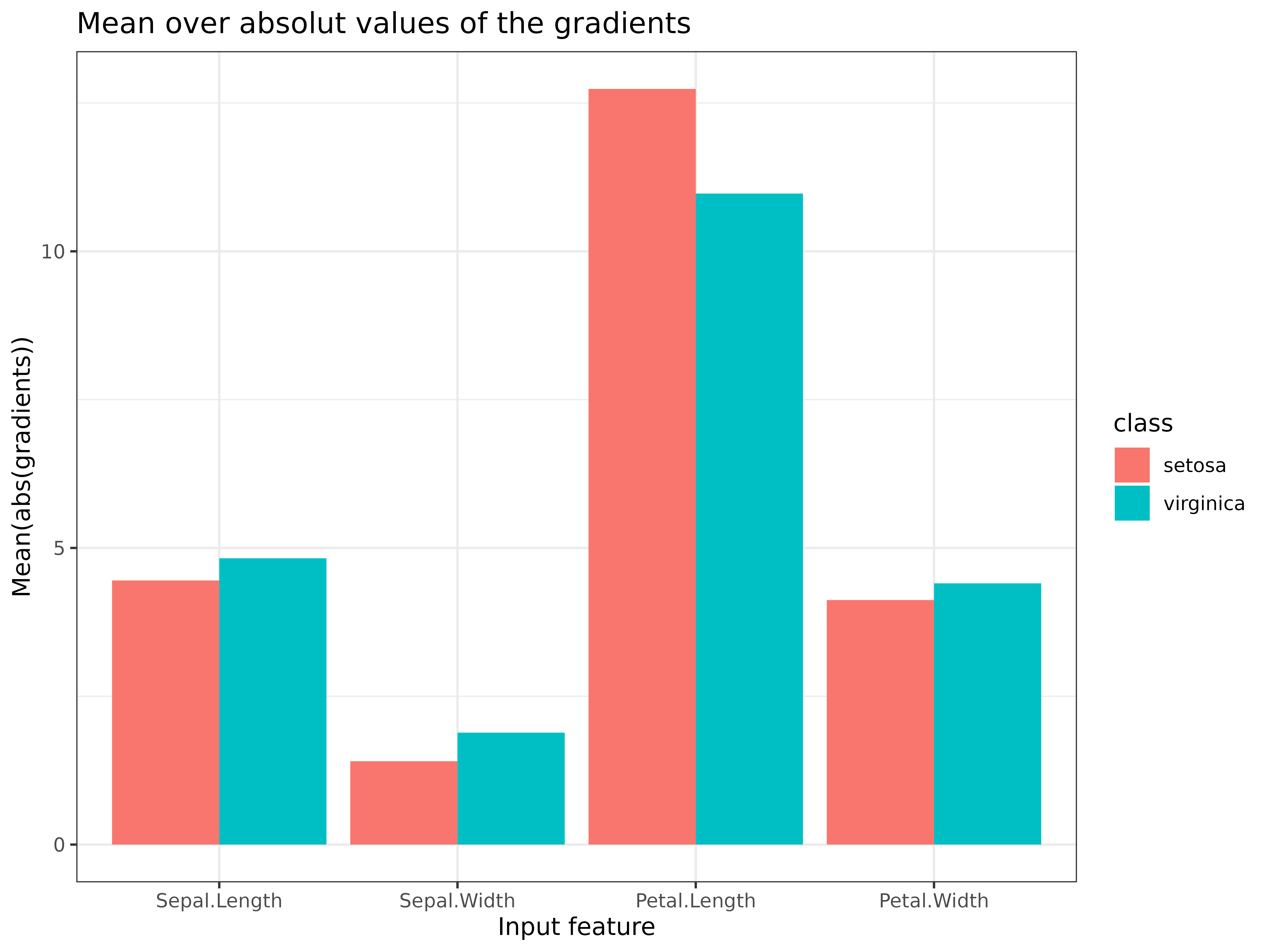

Plot single results plot()

This method visualizes the result of the selected method and enables a in-depth visual investigation with the help of the S4 classes innsight_ggplot2 and innsight_plotly. You can use the argument data_idx to select the data points in the given data for the plot. In addition, the individual plot’s output nodes or classes can be selected with the argument output_idx (for indices) or output_label (for the class labels). But this has to be a subset of the argument output_idx or output_label passed to the respective method previously because the results were only calculated for these outputs. The different results for the selected data points and outputs are visualized using the ggplot2-based S4 class innsight_ggplot2. You can also use the as_plotly argument to generate an interactive plot with innsight_plotly based on the plot function plotly::plot_ly. For more information and the whole bunch of possibilities, see the R documentation (?innsight_ggplot2 and ?innsight_plotly) or in this section. There are the following arguments:

• data_idx: An integer vector containing the numbers of the data points whose result is to be plotted, e.g., c(1,3) for the first and third data point in the given data.

  📝 Note
  This argument will be ignored for the global Connection Weights method.

• output_idx: The indices of the output nodes for which the results is to be plotted. This can be either a vector of indices or a list of vectors of indices but must be a subset of the indices for which the results were calculated, i.e., a subset of the argument output_idx passed to the respective method previously. By default (NULL), the smallest index of all calculated output nodes and output layers is used.
• output_label: The labels of the output nodes for which the results is to be plotted. This can be either a vector of labels or a list of vectors of labels (character or factor) but must be a subset of the labels for which the results were calculated, i.e., a subset of the argument output_label passed to the respective method previously. By default (NULL), the smallest index of all calculated output nodes and output layers is used.

• aggr_channels: Pass one of 'norm', 'sum', 'mean' or a custom function to aggregate the channels. By default ('sum'), the sum of all channels is used.

  📝 Note
  This argument is used only for 1D signal and 2D image input data.

• as_plotly: This logical value (default: FALSE) can be used to create an interactive plot based on the library plotly (see ?innsight_plotly or here for details).

  📝 Note
  Make sure that the suggested package plotly is installed in your R session.

• same_scale: A logical value that specifies whether the individual plots have the same fill scale across multiple input layers or whether each is scaled individually. This argument is only used if more than one input layer’s result is plotted. This is especially relevant when plotting explanations of images and tabular data simultaneously since the relevances are usually from different scales.

  📝 Note
  By default, the relevances within each output class, data point, and, if available, input layer are scaled and highlighted separately with the colors red for positive, blue for negative, and white for the absence of relevance so that the different intensities of the relevances can be distinguished by their colors.

• show_preds: This logical value indicates whether the plots display the prediction, the sum of calculated relevances, and, if available, the targeted decomposition value in a small infobox. For example, in the case of Gradient$\times$Input, the goal is to obtain a feature-wise decomposition of the predicted value, while for DeepLift and IntegratedGradient, the goal is the difference between the prediction and the reference value, i.e., $f(x) - f(\tilde{x})$. However, the infoboxes are only shown for ggplo2-based plots.

# Class method
method$plot(
  data_idx = 1,
  output_idx = NULL,
  output_label = NULL,
  aggr_channels = "sum",
  as_plotly = FALSE,
  same_scale = FALSE,
  show_preds = TRUE
)

# or the S3 method
plot(method,
  data_idx = 1,
  output_idx = NULL,
  output_label = NULL,
  aggr_channels = "sum",
  as_plotly = FALSE,
  same_scale = FALSE,
  show_preds = TRUE
)

Examples and usage:

# Create plot for output classes 'setosa' and  'virginica' and
# data points '1' and '70'
p <- plot(tab_grad, output_label = c("setosa", "virginica"), data_idx = c(1, 70))

# Although it's not a ggplot2 object ...
class(p)
#> [1] "innsight_ggplot2"
#> attr(,"package")
#> [1] "innsight"

# ... it can be treated as one
p +
  ggplot2::theme_bw() +
  ggplot2::ggtitle("My first 'innsight'-plot")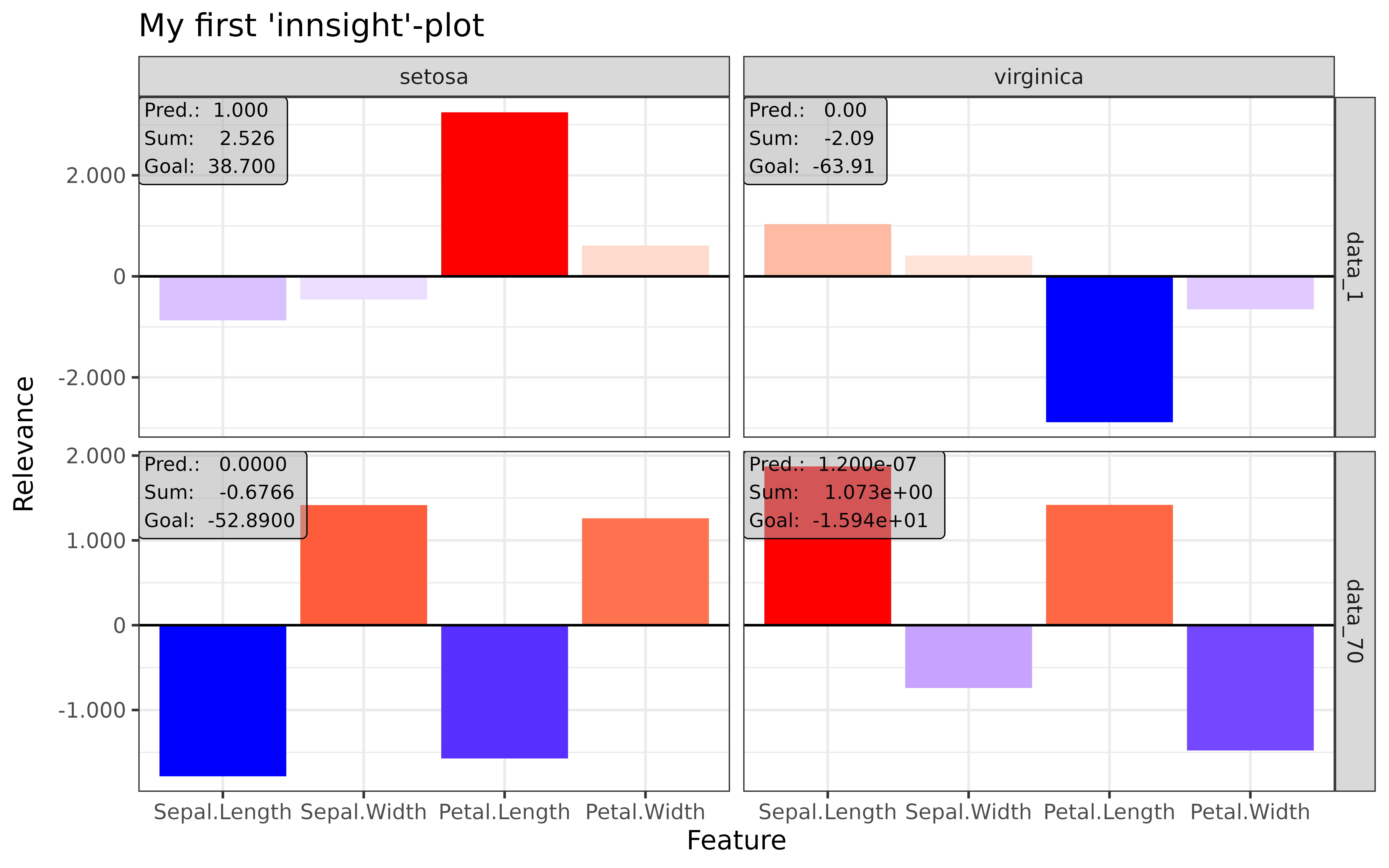

# In addition, you can use all the options of the class 'innsight_ggplot2',
# e.g. getting the corresponding ggplot2 object
class(p[[1, 1]])
#> [1] "gg"     "ggplot"

# or creating a subplot
p[2, 1:2]

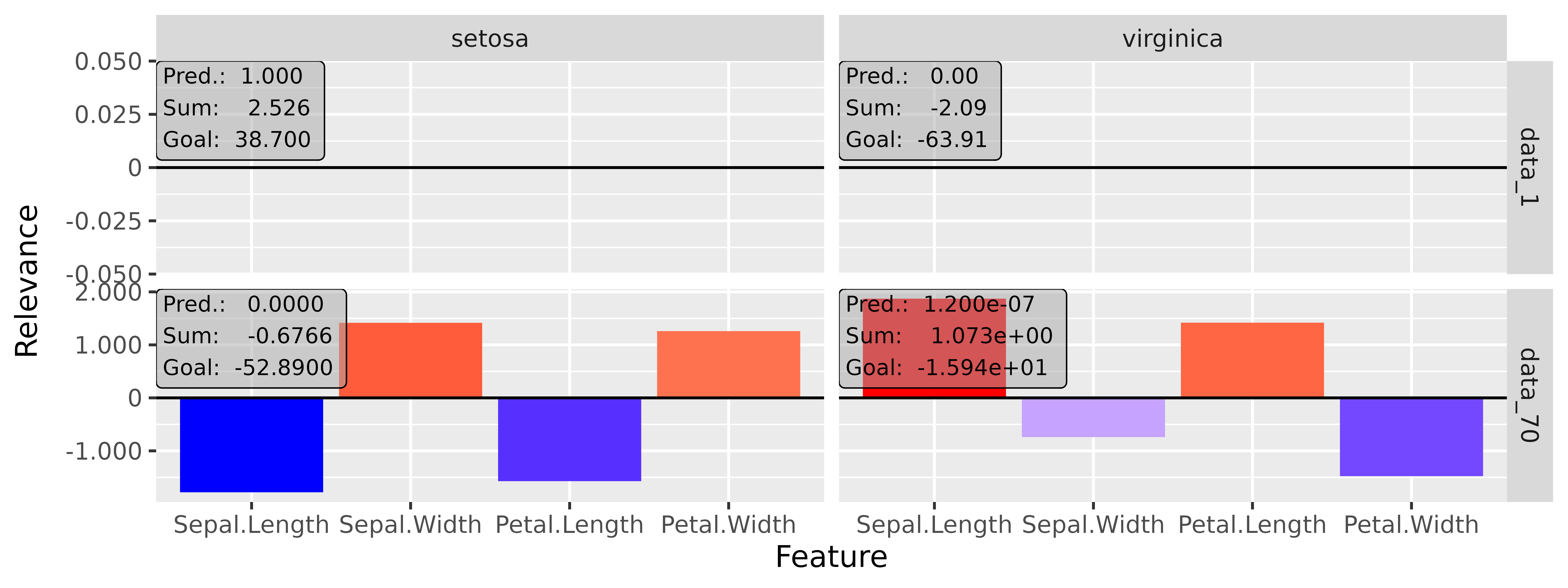
# You can do the same with the plotly-based plots
p <- plot(tab_grad, output_idx = c(1, 3), data_idx = c(1, 70), as_plotly = TRUE)

# Show plot (it also includes a drop down menu for selecting the colorscale)
p

# We can do the same for models with image data. In addition, you can define
# the aggregation function for the channels
p <- plot(img_grad,
  output_idx = c(1, 2), data_idx = c(1, 4),
  aggr_channels = "norm"
)

# Although it's not a ggplot2 object ...
class(p)
#> [1] "innsight_ggplot2"
#> attr(,"package")
#> [1] "innsight"

# ... it can be treated as one
p +
  ggplot2::theme_bw() +
  ggplot2::scale_fill_viridis_c() +
  ggplot2::ggtitle("My first 'innsight'-plot")
#> Scale for fill is already present.
#> Adding another scale for fill, which will replace the existing scale.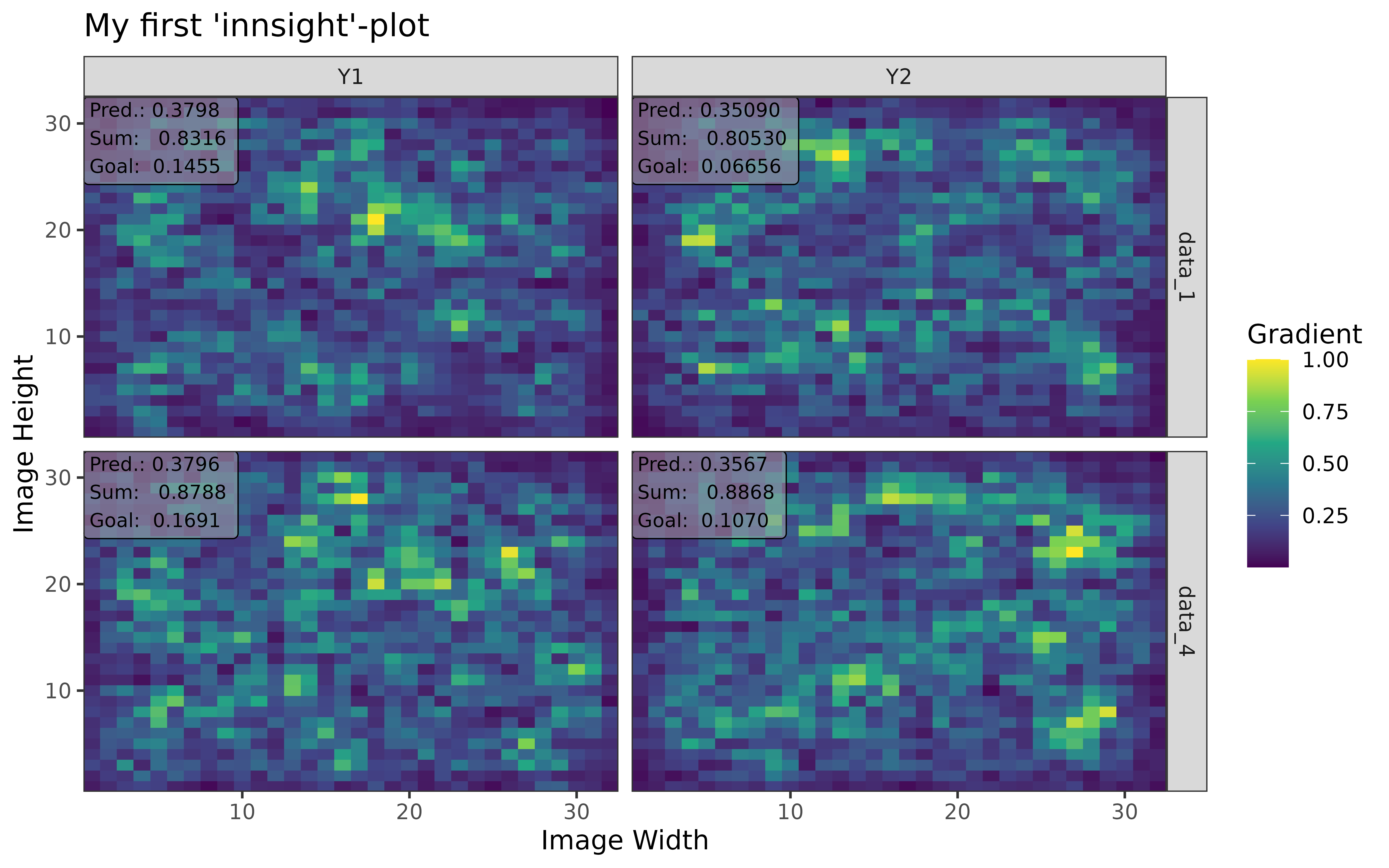

If you want to make changes to the results before plotting, you can get the results with method$result (a list of torch_tensors!), change it accordingly, and then save it back to the field method$result as a list of torch_tensors.

# You can also do custom modifications of the results, e.g.
# taking the absolute value of all results. But the
# shape has to be the same after the modification!
result <- tab_grad$result

# The model has only one input (inner list) and one output layer (outer list), so
# we need to modify only a single entry
str(result)
#> List of 1
#>  $ :List of 1
#>   ..$ :Float [1:150, 1:4, 1:2]

# Take the absolute value and save it back to the object 'img_grad'
tab_grad$result[[1]][[1]] <- abs(result[[1]][[1]])

# Show the result
plot(tab_grad, output_idx = c(1, 3), data_idx = c(1, 70))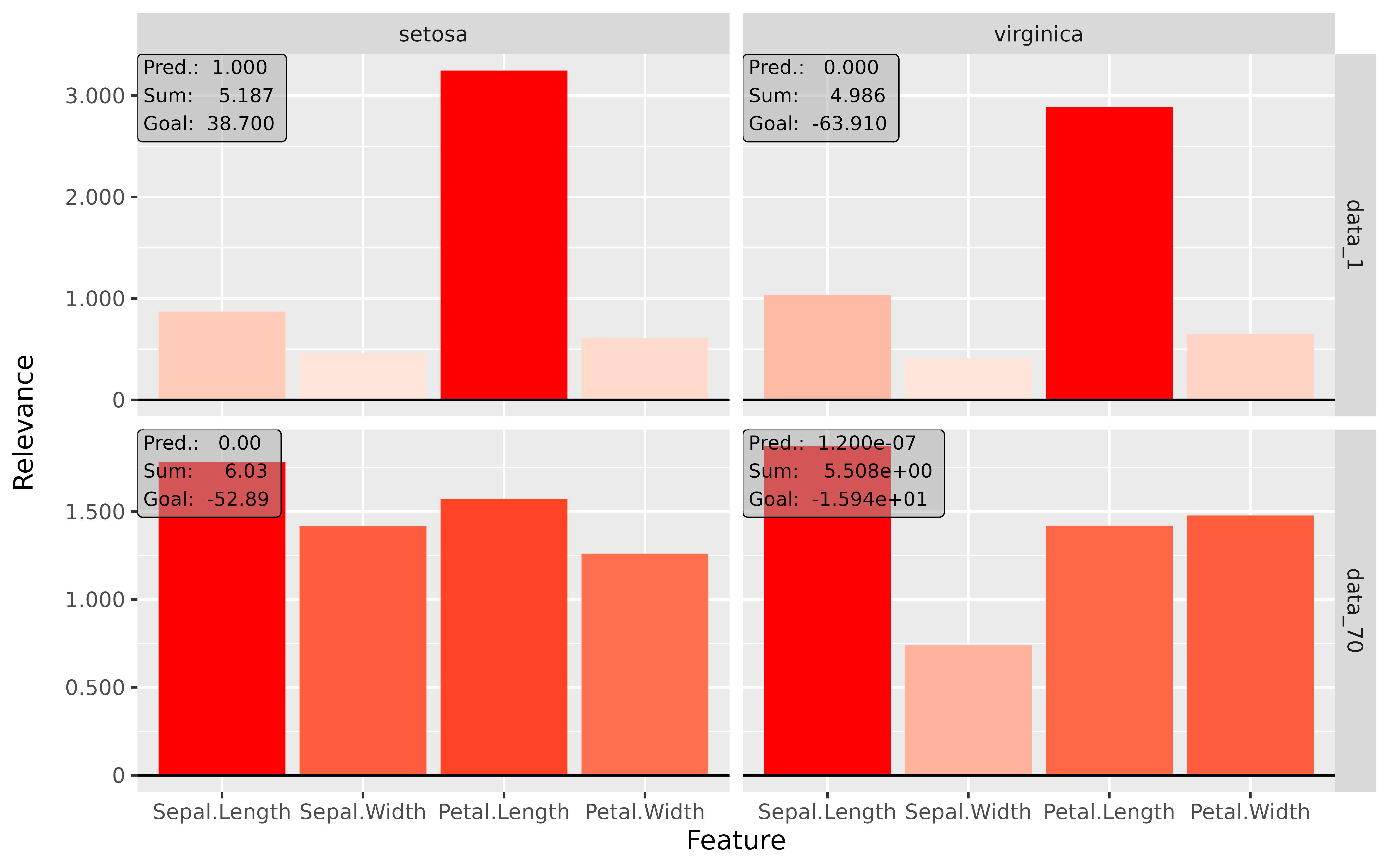

Plot summarized results plot_global()

This method visualizes summarized results of the selected method over all data points (or a subset) and enables an in-depth visual investigation with the help of the S4 classes innsight_ggplot2 and innsight_plotly similar to the previous plot function. You can use the argument output_idx/output_label to select the individual output nodes for the plot. But this has to be a subset of the argument output_idx or output_label passed to the respective method previously because the results were only calculated for these outputs. For tabular and 1D signal data, boxplots are created in which a reference value can be selected from the data using the ref_data_idx argument. For images, only the pixel-wise median is visualized due to the complexity. The different results for the selected outputs are visualized using the ggplot2-based S4 class innsight_ggplot2. You can also use the as_plotly argument to generate an interactive plot with innsight_plotly based on the plot function plotly::plot_ly. For more information and the whole bunch of possibilities, see the R documentation (?innsight_ggplot2 and ?innsight_plotly) or in this section.

There are the following arguments:

• output_idx: The indices of the output nodes for which the results is to be plotted. This can be either a vector of indices or a list of vectors of indices but must be a subset of the indices for which the results were calculated, i.e., a subset of the argument output_idx passed to the respective method previously. By default (NULL), the smallest index of all calculated output nodes and output layers is used.
• data_idx: By default, all available data points are used to calculate the boxplot information. However, this parameter can be used to select a subset of them by passing the indices. For example, with c(1:10, 25, 26) only the first 10 data points and the 25th and 26th are used to calculate the boxplots.
• output_label: The labels of the output nodes for which the results is to be plotted. This can be either a vector of labels or a list of vectors of labels (character or factor) but must be a subset of the labels for which the results were calculated, i.e., a subset of the argument output_label passed to the respective method previously. By default (NULL), the smallest index of all calculated output nodes and output layers is used.

• ref_data_idx: This integer number determines the index for the reference data point. In addition to the boxplots, it is displayed in red color and is used to compare an individual result with the summary statistics provided by the boxplot. With the default value (NULL), no individual data point is plotted. This index can be chosen with respect to all available data, even if only a subset is selected with argument data_idx.

  📝 Note
  Because of the complexity of 2D image inputs, this argument is used only for tabular and 1D signal data and disregarded for images.

• aggr_channels: Pass one of 'norm', 'sum', 'mean' or a custom function to aggregate the channels. By default ('sum'), the sum of all channels is used.

  📝 Note
  This argument is used only for 1D signal and 2D image input data.

• preprocess_FUN: This function is applied to the method’s result before calculating the boxplot information or medians. Since positive and negative values often cancel each other out, the absolute value is used by default. But you can also use the raw results (base::identity) to see the results’ orientation, the squared data (function(x) x^2) to weight the outliers higher or any other function.

• as_plotly: This logical value (default: FALSE) can be used to create an interactive plot based on the library plotly (see ?innsight_plotly or here for details).

  📝 Note
  Make sure that the suggested package plotly is installed in your R session.

• individual_data_idx (only relevant for a plotly plot with tabular or 1D signal inputs!): This integer vector of data indices determines the available data points in a dropdown menu, which are drawn individually analogous to ref_data_idx only for more data points. With the default value NULL, the first individual_max data points are used.

  📝 Note
  If ref_data_idx is specified, this data point will be added to those from individual_data_idx in the dropdown menu.

• individual_max (only relevant for a plotly plot with tabular or 1D signal inputs!): This integer determines the maximum number of individual data points in the dropdown menu without counting ref_data_idx. This means that if individual_data_idx has more than individual_max indices, only the first individual_max will be used. A too high number can significantly increase the runtime.

# Class method
method$plot_global(
  output_idx = NULL,
  data_idx = "all",
  ref_data_idx = NULL,
  aggr_channels = "sum",
  preprocess_FUN = abs,
  as_plotly = FALSE,
  individual_data_idx = NULL,
  individual_max = 20
)

# or the S3 method
plot_global(method,
  output_idx = NULL,
  data_idx = "all",
  ref_data_idx = NULL,
  aggr_channels = "sum",
  preprocess_FUN = abs,
  as_plotly = FALSE,
  individual_data_idx = NULL,
  individual_max = 20
)

# or the alias for tabular or signal data
boxplot(...)

Examples and usage:

# Create a boxplot for output classes '1' (setosa) and '3' (virginica)
p <- boxplot(tab_grad, output_idx = c(1, 3))

# Although, it's not a ggplot2 object ...
class(p)
#> [1] "innsight_ggplot2"
#> attr(,"package")
#> [1] "innsight"

# ... it can be treated as one
p +
  ggplot2::theme_bw() +
  ggplot2::ggtitle("My first 'innsight'-boxplot!")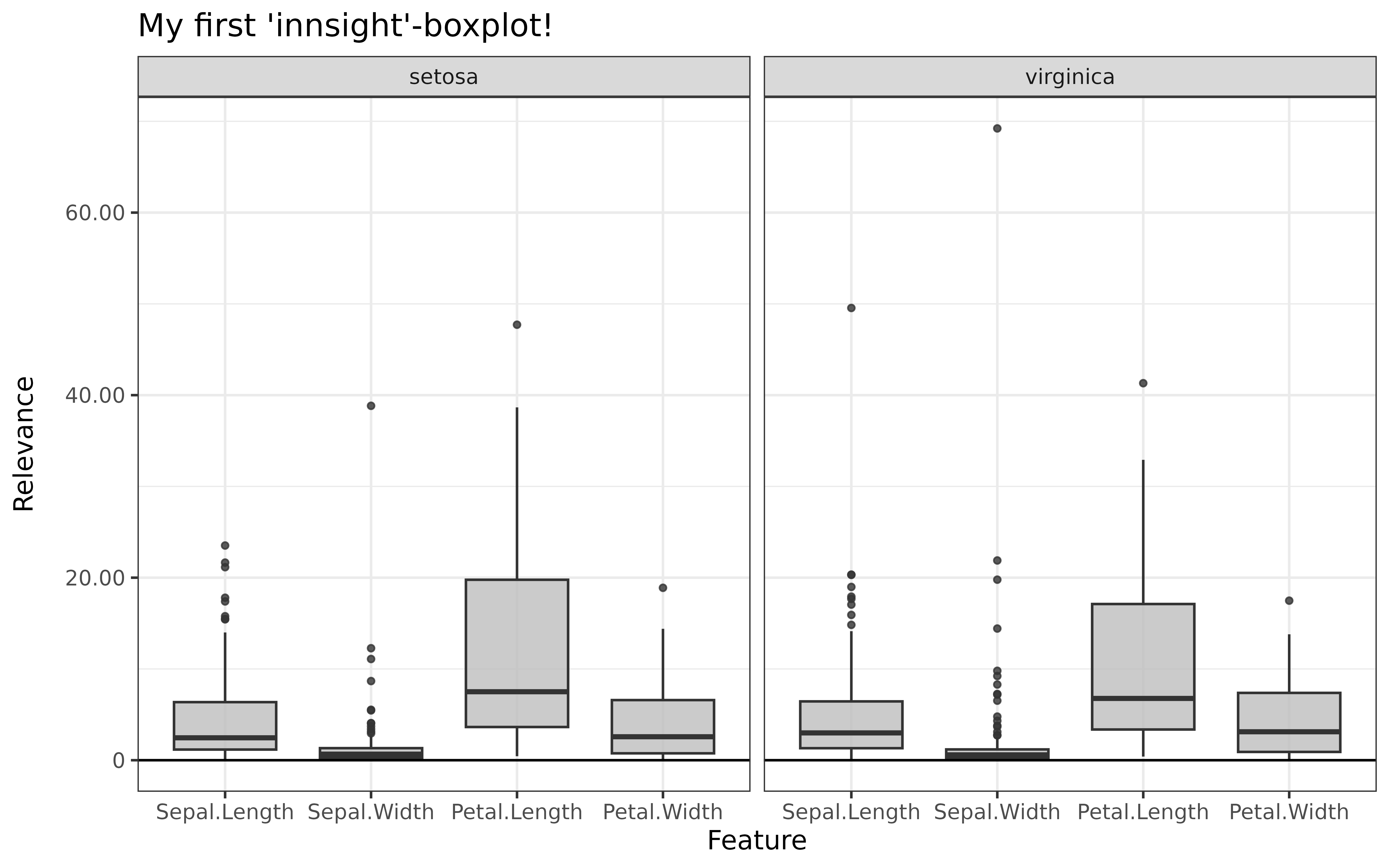

# You can also select only the indices of the class 'setosa'
# and add a reference data point of another class ('versicolor')
boxplot(tab_grad, output_idx = c(1, 3), data_idx = 1:50, ref_data_idx = c(60))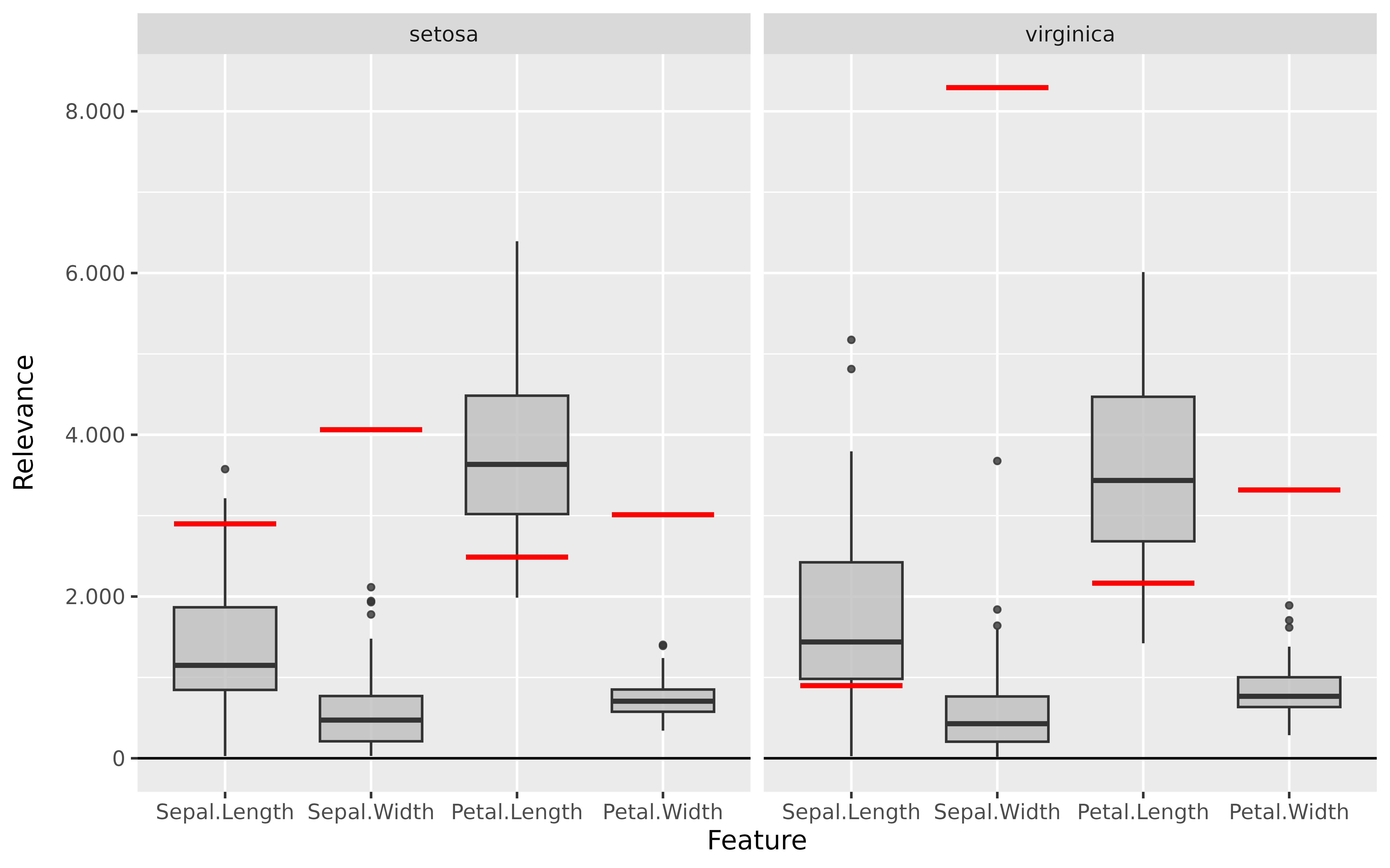

# You can do the same with the plotly-based plots
p <- boxplot(tab_grad,
  output_idx = c(1, 3), data_idx = 1:50,
  ref_data_idx = 60, as_plotly = TRUE
)

# Show plot (it also includes a drop down menu for selecting the reference data
# point and toggle the plot type 'Boxplot' or 'Violin')
p

# We can do the same for models with image data (but have to use the method
# `plot_global`, since no boxplots are created). In addition, you can define
# the aggregation function for the channels
p <- plot_global(img_grad, output_idx = c(1, 2), aggr_channels = "norm")

# Although it's not a ggplot2 object ...
class(p)
#> [1] "innsight_ggplot2"
#> attr(,"package")
#> [1] "innsight"

# ... it can be treated as one
p +
  ggplot2::theme_bw() +
  ggplot2::coord_flip() +
  ggplot2::ggtitle("My first 'innsight'-boxplot")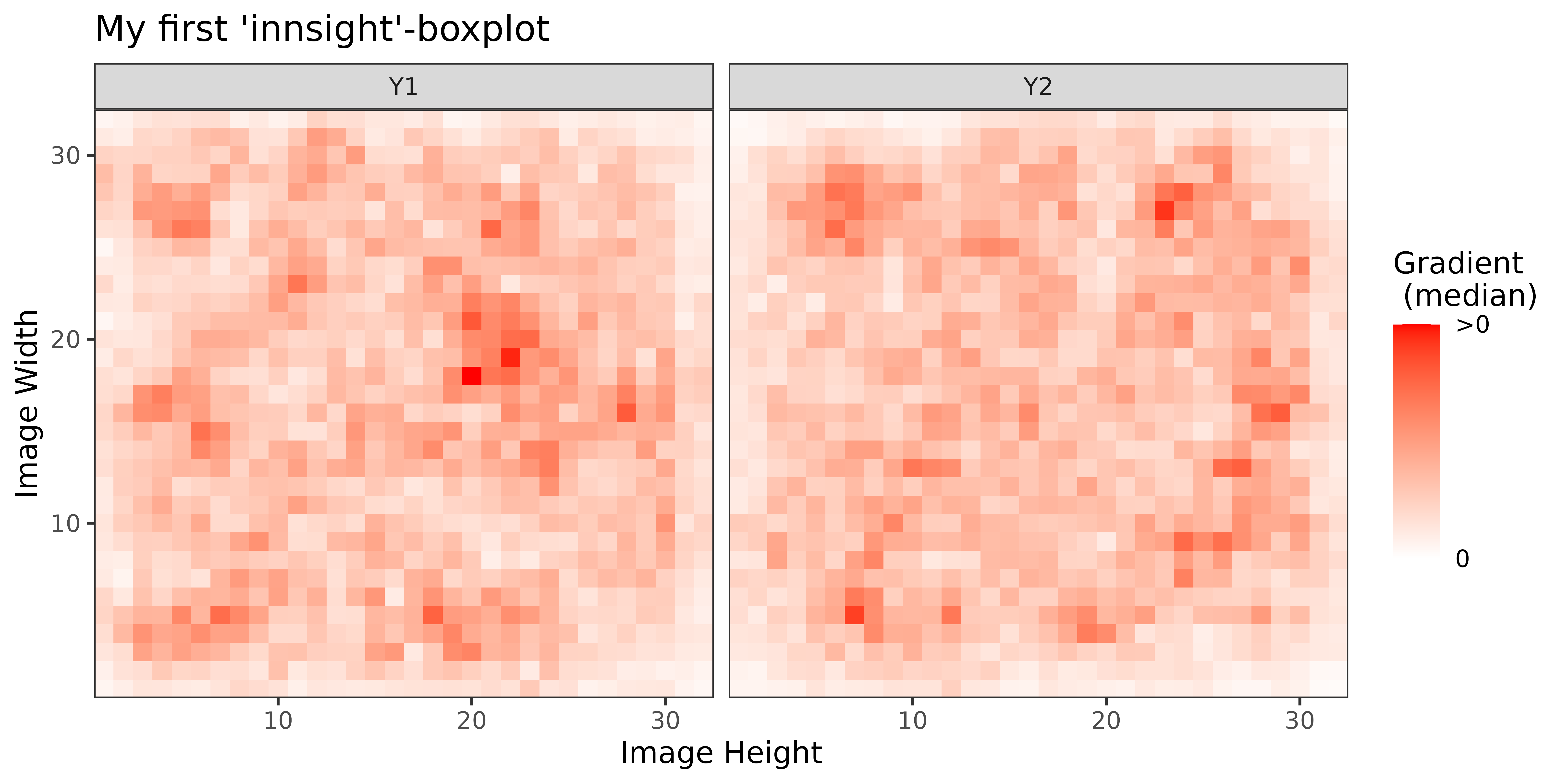

# You can do the same with the plotly-based plots
p <- plot_global(img_grad,
  output_idx = c(1, 2), aggr_channels = "norm",
  as_plotly = TRUE
)

# Show plot (it also includes a drop down menu for selecting the colorscale,
# another menu for toggling between the plot types 'Heatmap' and 'Contour'
# and a scale for selecting the respective percentile)
p

Advanced plotting

In the preceding two sections, the basic plot() and plot_global()/boxplot() functions have already been explained. As mentioned there, these functions create either an object of the S4 class innsight_ggplot2 (if as_plotly = FALSE) or one of the S4 class innsight_plotly (if as_plotly = TRUE). These are intended as a generalization of the usual ggplot2 or plotly objects since, with these packages, one quickly reaches their limits of clear visualization possibilities for models with multiple input and/or output layers. For example, two plots with different x-axis scales for each output node need to be generated in a model with images and tabular data as inputs.

Create results for the following examples

library(keras)
library(torch)

# Create model with tabular data as inputs and one output layer
model <- keras_model_sequential() %>%
  layer_dense(50, activation = "relu", input_shape = c(5)) %>%
  layer_dense(20, activation = "relu") %>%
  layer_dense(3, activation = "softmax")

converter <- convert(model)

data <- array(rnorm(5 * 50), dim = c(50, 5))
res_simple <- run_grad(converter, data)

# Create model with images as inputs and two output layers
input_image <- layer_input(shape = c(10, 10, 3))
conv_part <- input_image %>%
  layer_conv_2d(5, c(2, 2), activation = "relu", padding = "same") %>%
  layer_average_pooling_2d() %>%
  layer_conv_2d(4, c(2, 2)) %>%
  layer_activation(activation = "softplus") %>%
  layer_flatten()

output_1 <- conv_part %>%
  layer_dense(50, activation = "relu") %>%
  layer_dense(3, activation = "softmax")

output_2 <- conv_part %>%
  layer_dense(50, activation = "relu") %>%
  layer_dense(3, activation = "softmax")

keras_model_concat <- keras_model(
  inputs = input_image,
  outputs = c(output_1, output_2)
)

converter <- convert(keras_model_concat)
#> Skipping InputLayer ...

data <- array(rnorm(10 * 10 * 3 * 5), dim = c(5, 10, 10, 3))
res_one_input <- run_grad(converter, data,
  channels_first = FALSE,
  output_idx = list(1:3, 1:3)
)

# Create model with images and tabular data as inputs and two
# output layers
input_image <- layer_input(shape = c(10, 10, 3))
input_tab <- layer_input(shape = c(10))

conv_part <- input_image %>%
  layer_conv_2d(5, c(2, 2), activation = "relu", padding = "same") %>%
  layer_average_pooling_2d() %>%
  layer_conv_2d(4, c(2, 2)) %>%
  layer_activation(activation = "softplus") %>%
  layer_flatten()

output_1 <- layer_concatenate(list(conv_part, input_tab)) %>%
  layer_dense(50, activation = "relu") %>%
  layer_dropout(0.3) %>%
  layer_dense(3, activation = "softmax")

output_2 <- layer_concatenate(list(conv_part, input_tab)) %>%
  layer_dense(3, activation = "softmax")

keras_model_concat <- keras_model(
  inputs = list(input_image, input_tab),
  outputs = list(output_1, output_2)
)

converter <- convert(keras_model_concat)
#> Skipping InputLayer ...
#> Skipping InputLayer ...
#> Skipping Dropout ...

data <- lapply(list(c(10, 10, 3), c(10)), function(x) torch_randn(c(5, x)))
res_two_inputs <- run_grad(converter, data,
  times_input = TRUE,
  channels_first = FALSE,
  output_idx = list(1:3, 1:3)
)

Plots based on ggplot2

All ggplot2-based plots generated by the innsight package are an object of the S4 class innsight_ggplto2, a simple extension of a ggplot2 object that enables more detailed analysis and comparison of the results. In addition, it provides a way to visualize the results of models with multiple input or output layers with different scales, e.g., images and tabular data. The values in the slots of this class depend very much on whether results for multiple input or output layers (multiplot = TRUE), or for only a single input and output layer (multiplot = FALSE) are visualized as described in the following. But in general, however, the slots are only explained here for internal purposes and should not be changed in standard use cases.

Results for a single input and output layer

If the model passed to a method from the innsight package has only one input layer, or the results to be plotted are only from a single output layer (i.e., slot multiplot = FALSE), the S4 class innsight_ggplot2 is just a wrapper of a single ggplot2 object. This object is stored as a 1x1 matrix in the slot grobs and the slots output_strips and col_dims contain only empty lists because no second line of stripes describing the input or output layer is needed.

Slots:

• grobs: A 1x1 matrix containing the whole ggplot2 object.

• mulitplot: In this case, this logical value is always FALSE.

• output_strips: In this case, this value is an empty list list().

• col_dims: In this case, this value is an empty list list().

• boxplot: A logical value indicating whether the result of individual data points or a boxplot over multiple instances is displayed.

# Create plot for output node 1 and 2 in the first output layer and
# data points 1 and 3
p <- plot(res_one_input, output_idx = c(1, 2), data_idx = c(1, 3))

# It's not an ggplot2 object
class(p)
#> [1] "innsight_ggplot2"
#> attr(,"package")
#> [1] "innsight"

# The slot 'grobs' only contains a single entry
p@grobs
#>      [,1] 
#> [1,] gg,11

# It's not a multiplot
p@multiplot
#> [1] FALSE

# Therefore, slots 'output_strips' and 'col_dims' are empty lists
p@output_strips
#> list()
p@col_dims
#> list()

Although it is an object of the class innsight_ggplot2, the generic function +.innsight_ggplot2 provides a ggplot2-typical usage to modify the representation. The graphical objects are simply forwarded to the ggplot2 object stored in the slot grobs and added using ggplot2::+.gg (see ?ggplot2::`+.gg` for details). In addition, some generic functions are implemented to visualize or examine individual aspects of the overall plot in more detail. All available generic functions are listed below:

Available generic functions:

• + : This generic add function allows to treat an instance of innsight_ggplot2 as an ordinary plot object of ggplot2. For example geoms, themes and scales can be added as usual (see ggplot2::`+.gg` for more information). However, an object of the class innsight_ggplot2 is returned.
  Examples

  # Create plot
  p <- plot(res_one_input, output_idx = c(1, 2), data_idx = c(1, 3))
  
  # Now we can add geoms, themes and scales as usual for ggplot2 objects
  df <- data.frame(
    x = c(0.5, 0.5, 10.5, 10.5, 0.5),
    y = c(0.5, 10.5, 10.5, 0.5, 0.5)
  )
  new_p <- p +
    geom_path(df, mapping = aes(x = x, y = y), color = "red", size = 3) +
    theme_bw() +
    scale_fill_viridis_c()
  #> Scale for fill is already present.
  #> Adding another scale for fill, which will replace the existing scale.
  
  # This object is still an 'innsight_ggplot2' object...
  class(new_p)
  #> [1] "innsight_ggplot2"
  #> attr(,"package")
  #> [1] "innsight"
  
  # ... but all ggplot2 geoms, themes and scales are added
  new_p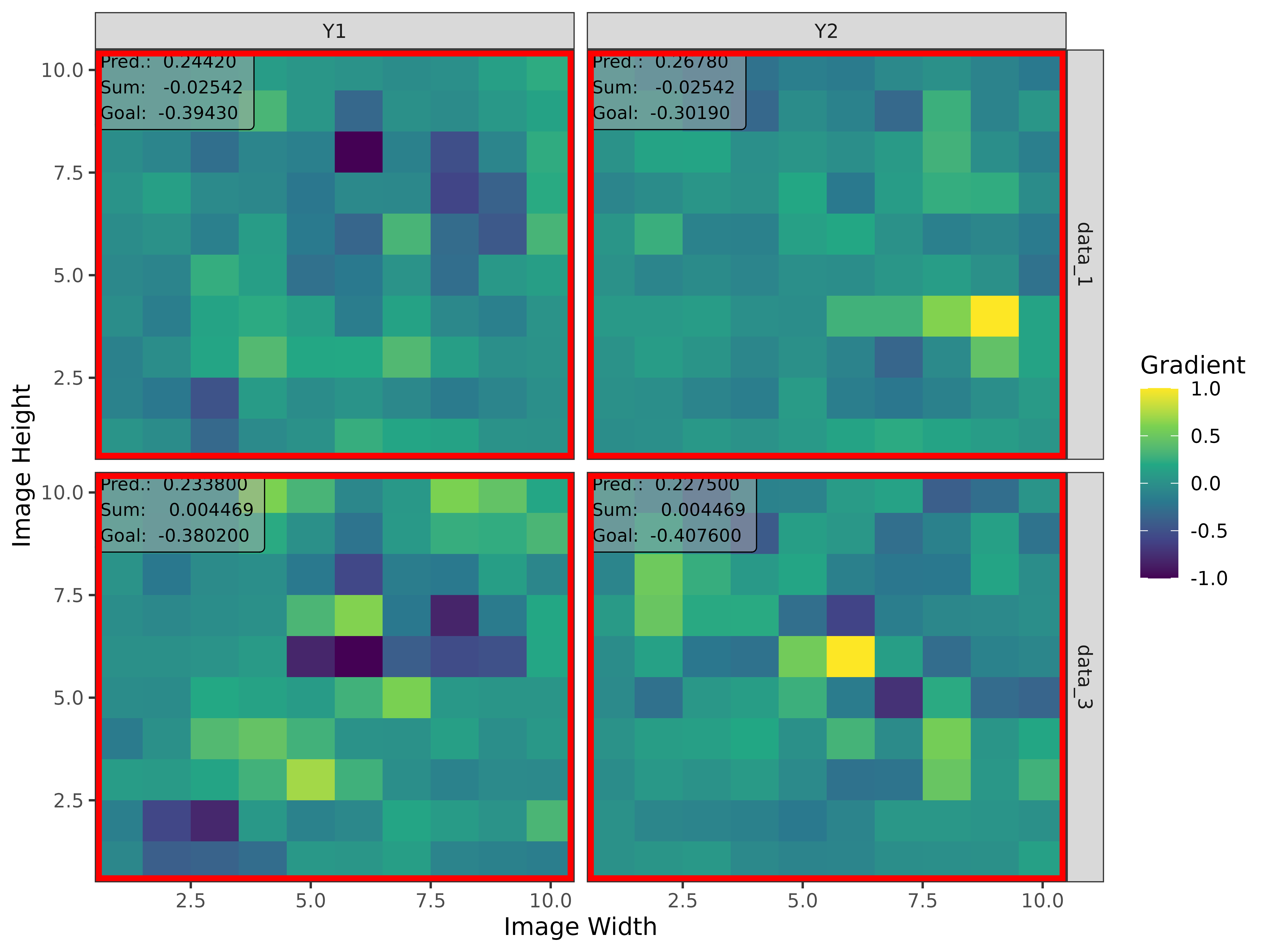

  

  # If the respective plot allows it, you can also use the already existing
  # mapping function and data:
  boxplot(res_simple, output_idx = 1:2) +
    geom_jitter(width = 0.3, alpha = 0.4)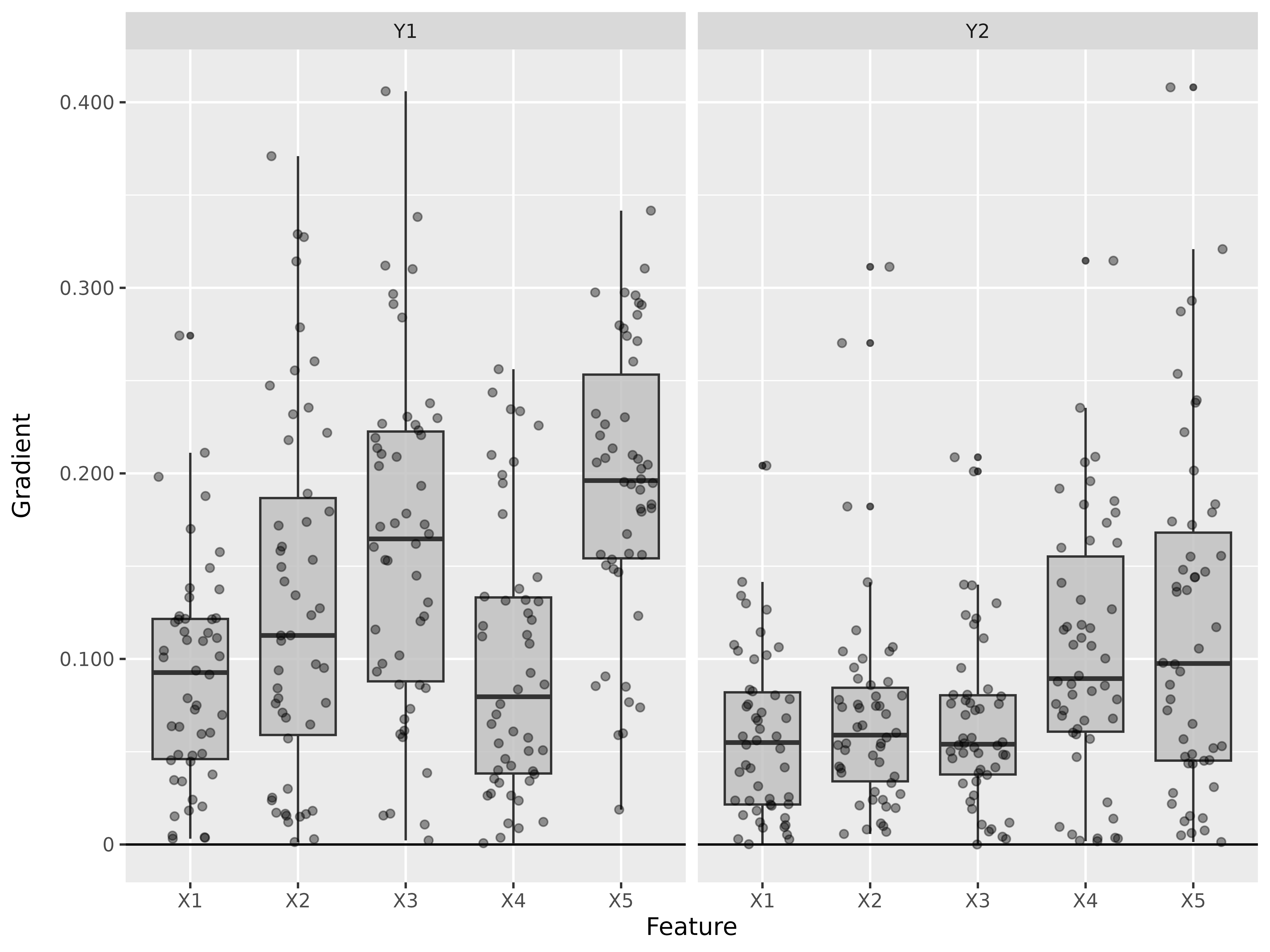

  
• [ : With this basic generic indexing functions, the plots of individual rows and columns can be accessed and is returned as an object of the class innsight_ggplot2.
  Example

  # Create plot
  p <- plot(res_one_input, output_idx = c(1, 2), data_idx = c(1, 3))
  
  # Show the whole plot
  p

  

  # Now you can select specific rows and columns for in-depth investigation,
  # e.g. only the result for output "Y1"
  p_new <- p[1:2, 1]
  
  # It's still an obeject of class 'innsight_ggplot2'
  class(p_new)
  #> [1] "innsight_ggplot2"
  #> attr(,"package")
  #> [1] "innsight"
  
  # Show the subplot
  p_new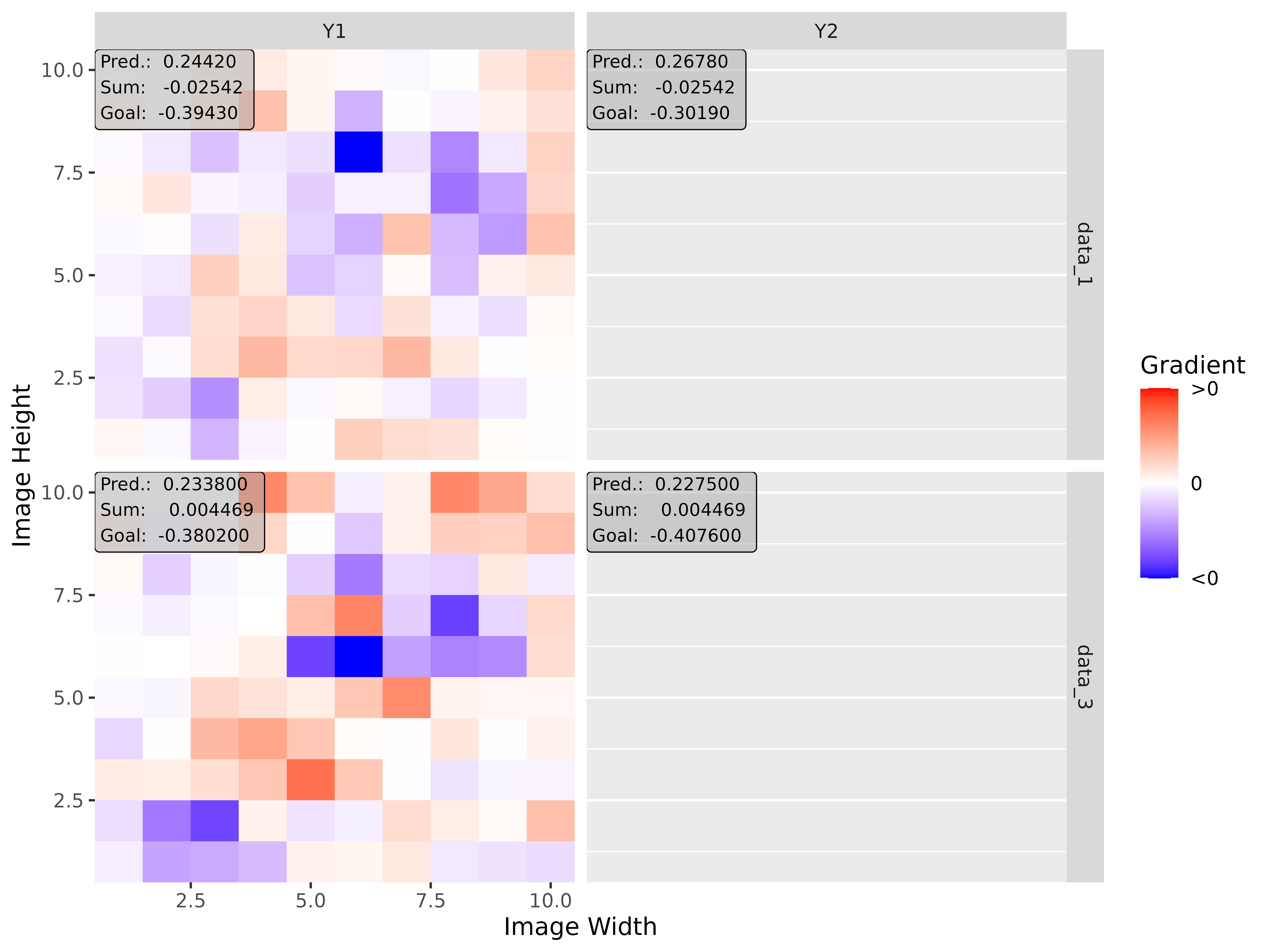

  
• [[ : With this basic generic indexing functions, you can select a single plot by passing the respective row and column index. This plot is returned as a ggplot2 object.
  Example

  # Create plot
  p <- plot(res_one_input, output_idx = c(1, 2), data_idx = c(1, 3))
  
  # Show the whole plot
  p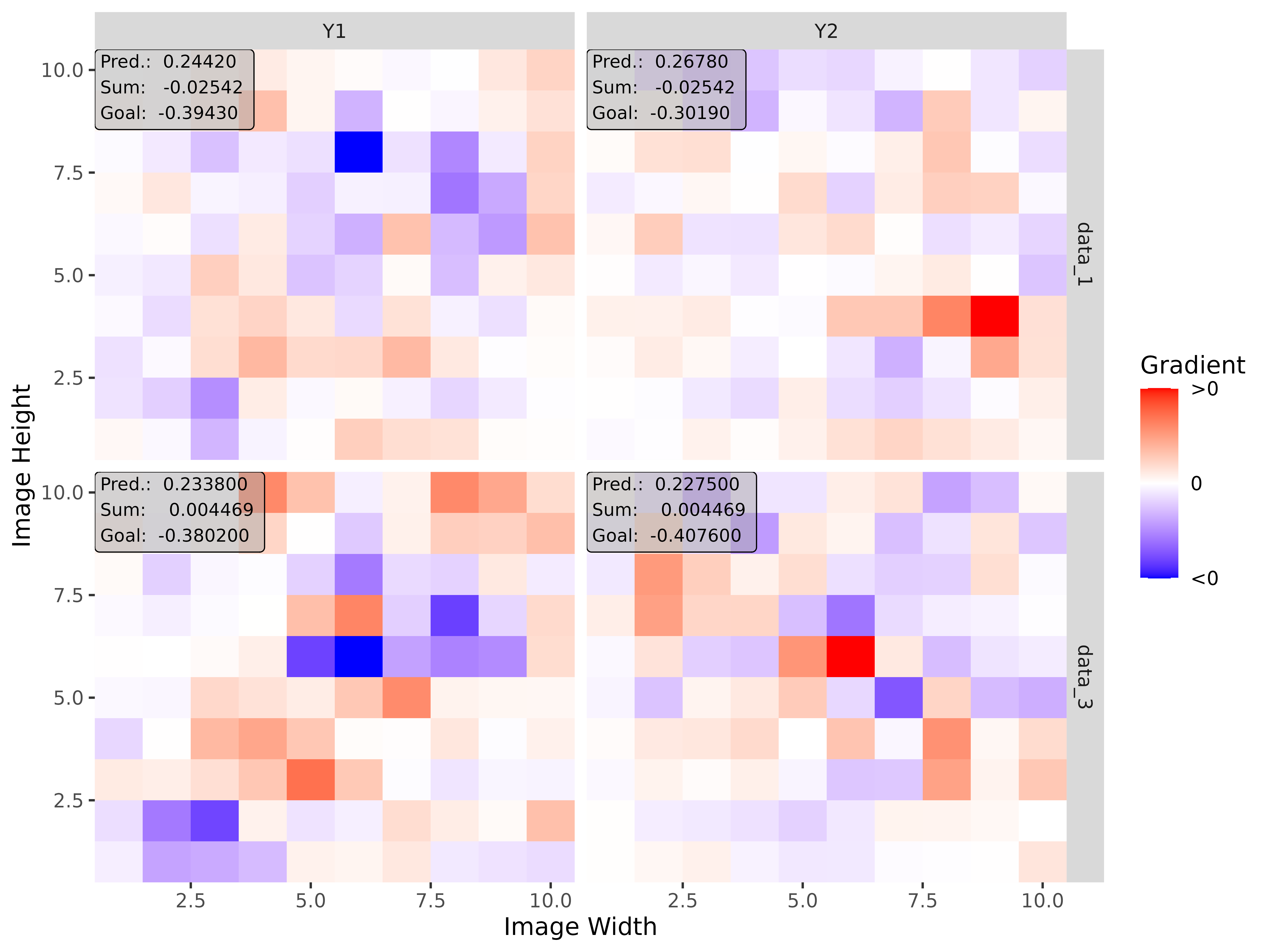

  

  # Now you can select a single plot by passing the row and column index,
  # e.g. the plot for output "Y1" and data point 3
  p_new <- p[[2, 1]]
  
  # This time a ggplot2 object is returned
  class(p_new)
  #> [1] "gg"     "ggplot"
  
  # Show the new plot
  p_new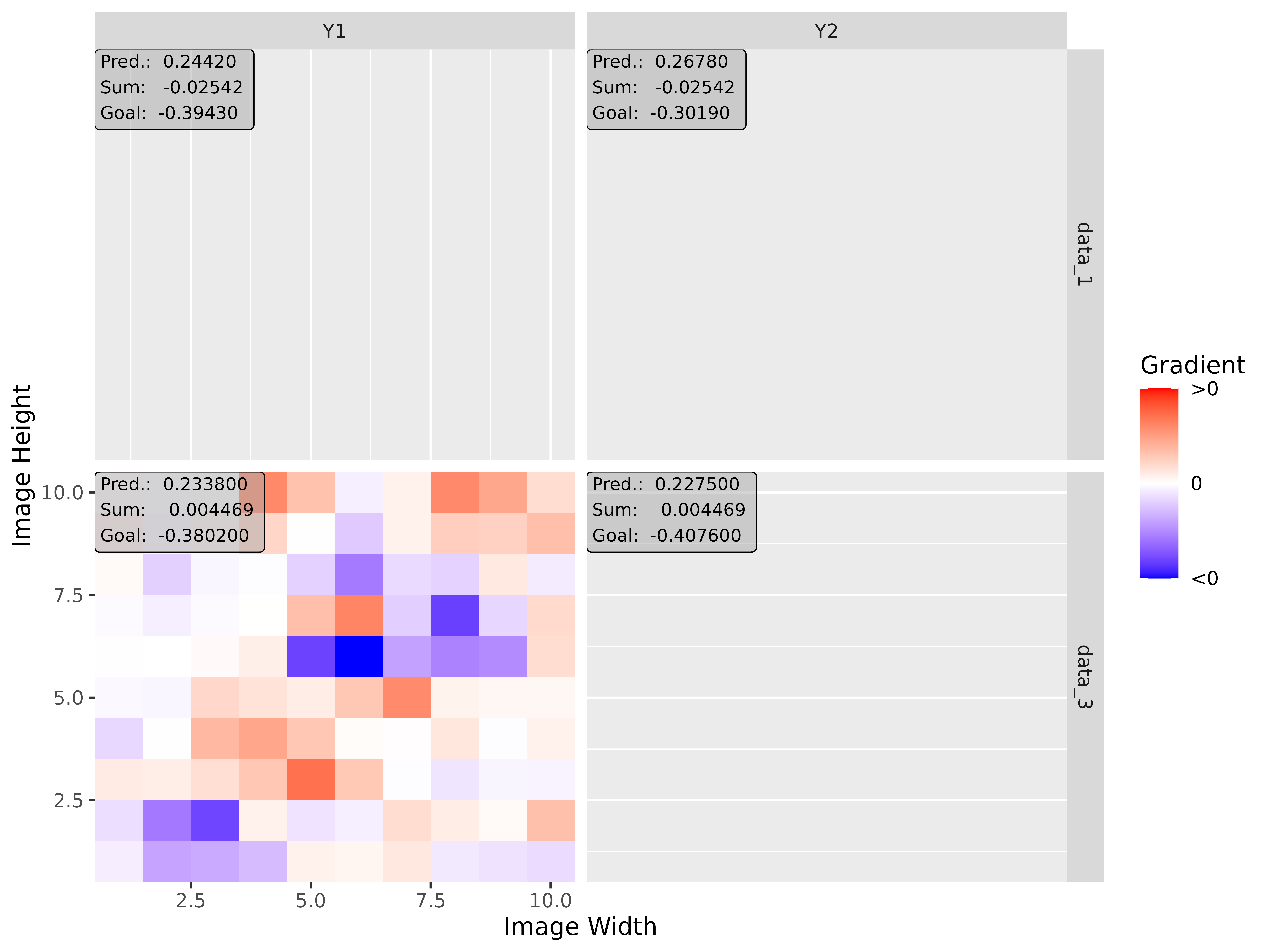

  
• plot, print and show : These methods provide generic visualization functions, which all behave the same in this case. They create the plot of the results and return a ggplot2 object invisibly.
  Examples

  # Create plot
  p <- plot(res_one_input, output_idx = c(1, 2), data_idx = 1)
  
  # All methods behave the same and return a ggplot2 object
  class(print(p))

  

  #> [1] "gg"     "ggplot"
  class(show(p))

  

  #> [1] "gg"     "ggplot"
  class(plot(p))

  

  #> [1] "gg"     "ggplot"

Results for multiple input and/or output layers

If the passed model has multiple input layers or results for multiple output layers are to be plotted, a ggplot2 object is created for each data point, input layer, and output node and then stored as a matrix in the slot grobs. During visualization, these are combined using the function gridExtra::arrangeGrob (see ?gridExtra::arrangeGrob for details) and corresponding strips for the output layer/node names are added at the top. The labels, column indices and theme for the extra row of strips are stored in the slots output_strips and col_dims. The strips for the input layer and the data points (if not a boxplot) are created using ggplot2::facet_grid in the individual ggplot2 objects of the grobs matrix. An example structure is shown below:

|      Output 1: Node 1      |      Output 1: Node 3      |
|   Input 1   |   Input 2    |   Input 1   |   Input 2    |
|---------------------------------------------------------|-------------
|             |              |             |              |
| grobs[1,1]  |  grobs[1,2]  | grobs[1,3]  | grobs[1,4]   | data point 1
|             |              |             |              |
|---------------------------------------------------------|-------------
|             |              |             |              |
| grobs[2,1]  |  grobs[2,2]  | grobs[2,3]  | grobs[2,4]   | data point 2
| 

Slots:

• grobs: The individual ggplot2 objects arranged as a matrix of size $\left(\text{N}_\text{datapoints}, \text{N}_\text{outputnodes} \cdot \text{N}_\text{inputlayers}\right)$.

• multiplot: In this case, this logical value is always TRUE.

• output_strips: This slot is a list containing the labels and themes of the strips for the output nodes, i.e., the additional strips at the top of the overall plot.

• col_dims: A list of the length of slot output_strips$labels assigning to each strip the number of columns for each output node strip.

• boxplot: A logical value indicating whether the result of individual data points or a boxplot over multiple instances is displayed.

📝 Note
Since these plots are more complex and do not build ggplot2 objects anymore, the suggested packages grid, gridExtra and gtable are needed and loaded.

# Create a plot for output node 1 in the first output layer and node 2 in the
# second output layer and data points 1 and 3
p <- plot(res_two_inputs, output_idx = list(1, c(1, 2)), data_idx = c(1, 3))
#> Loading required namespace: gridExtra

# It's not a ggplot2 object
class(p)
#> [1] "innsight_ggplot2"
#> attr(,"package")
#> [1] "innsight"

# In this case, 'grobs' is a 2x6 matrix
p@grobs
#>      [,1]  [,2]  [,3]  [,4]  [,5]  [,6] 
#> [1,] gg,11 gg,11 gg,11 gg,11 gg,11 gg,11
#> [2,] gg,11 gg,11 gg,11 gg,11 gg,11 gg,11

# It's a multiplot
p@multiplot
#> [1] TRUE

# Slot 'output_strips' is a list with the three labels for the output nodes
# and the theme for the strips
str(p@output_strips, max.level = 1)
#> List of 2
#>  $ labels:'data.frame':  3 obs. of  1 variable:
#>  $ theme :List of 136
#>   ..- attr(*, "class")= chr [1:2] "theme" "gg"
#>   ..- attr(*, "complete")= logi TRUE
#>   ..- attr(*, "validate")= logi TRUE

# Slot 'col_dims' contains the number of columns for each output node
p@col_dims
#> [[1]]
#> [1] 2
#> 
#> [[2]]
#> [1] 2
#> 
#> [[3]]
#> [1] 2

Analogous to the other case, the generic function +.innsight_ggplot2 provides a ggplot2-typical usage to modify the representation. The graphical objects are simply forwarded to the ggplot2 objects stored in the slot grobs and added using ggplot2::+.gg (see ?ggplot2::`+.gg` for details). In addition, some generic functions are implemented to visualize or examine individual aspects of the overall plot in more detail. All available generic functions are listed below:

• +, [ and [[ : These generic functions have the same behavior as in the upper case (see there for details and examples). Except for one additional argument in the indexing function [[, namely restyle. This argument can be used to decide whether the subplots are formatted according to the whole plot (i.e., labels, facet strips, etc., are transferred) or whether the subplot is extracted in the same way as it is shown in the whole plot.
  Example

  # Create plot
  p <- plot(res_two_inputs, output_idx = list(1, 2), data_idx = c(1,2))
  
  # Show the whole plot
  p

  

  # Select a restyled subplot (default)
  p[1, 1:2]

  

  # The same plot as shown in the whole plot
  p[1, 1:2, restyle = FALSE]

  
• plot, print and show : These methods provide generic visualization functions, which all behave the same in this case. They create the plot of the results and return a gtable object invisibly. For plot and print, you can also pass additional arguments forwarded to gridExtra::arrangeGrob.
  Examples

  # Create plot
  p <- plot(res_two_inputs, output_idx = list(1, 2), data_idx = 1)
  
  # All methods behave the same and return a ggplot2 object
  class(print(p))

  

  #> [1] "gtable" "gTree"  "grob"   "gDesc"
  class(show(p))

  

  #> [1] "gtable" "gTree"  "grob"   "gDesc"
  class(plot(p))

  

  #> [1] "gtable" "gTree"  "grob"   "gDesc"
  
  # You can also pass additional arguments to the method 'arrangeGrob',
  # e.g. double the width of both images
  print(p, widths = c(2, 1, 2, 1))

  
• [<- : Since, in this case, each plot from the slot grobs represents an independent plot, which are joined with arrageGrob, each plot can also be changed individually and is independent of the others. Individual modifications can be made with this generic function.
  Examples

  # Create plot
  p <- plot(res_two_inputs, output_idx = list(1, 2), data_idx = c(1, 3))
  
  # Remove colorbar in the plot for data point 3 and output 'Y1' in output
  # layer 1 (in such situations the `restyle` argument is useful)
  p[2, 1] <- p[2, 1, restyle = FALSE] + guides(fill = "none")
  
  # Change colorscale in the plot for data point 1 and output 'Y2' in output
  # layer 2
  p[1, 3:4] <- p[1, 3:4, restyle = FALSE] + scale_fill_gradient2(limit = c(-1, 1))
  #> Scale for fill is already present.
  #> Adding another scale for fill, which will replace the existing scale.
  #> Scale for fill is already present.
  #> Adding another scale for fill, which will replace the existing scale.
  
  # Change the theme in all plots for data point 3
  p[2, ] <- p[2, , restyle = FALSE] + theme_dark()
  
  # Show the result with all changes
  p

  

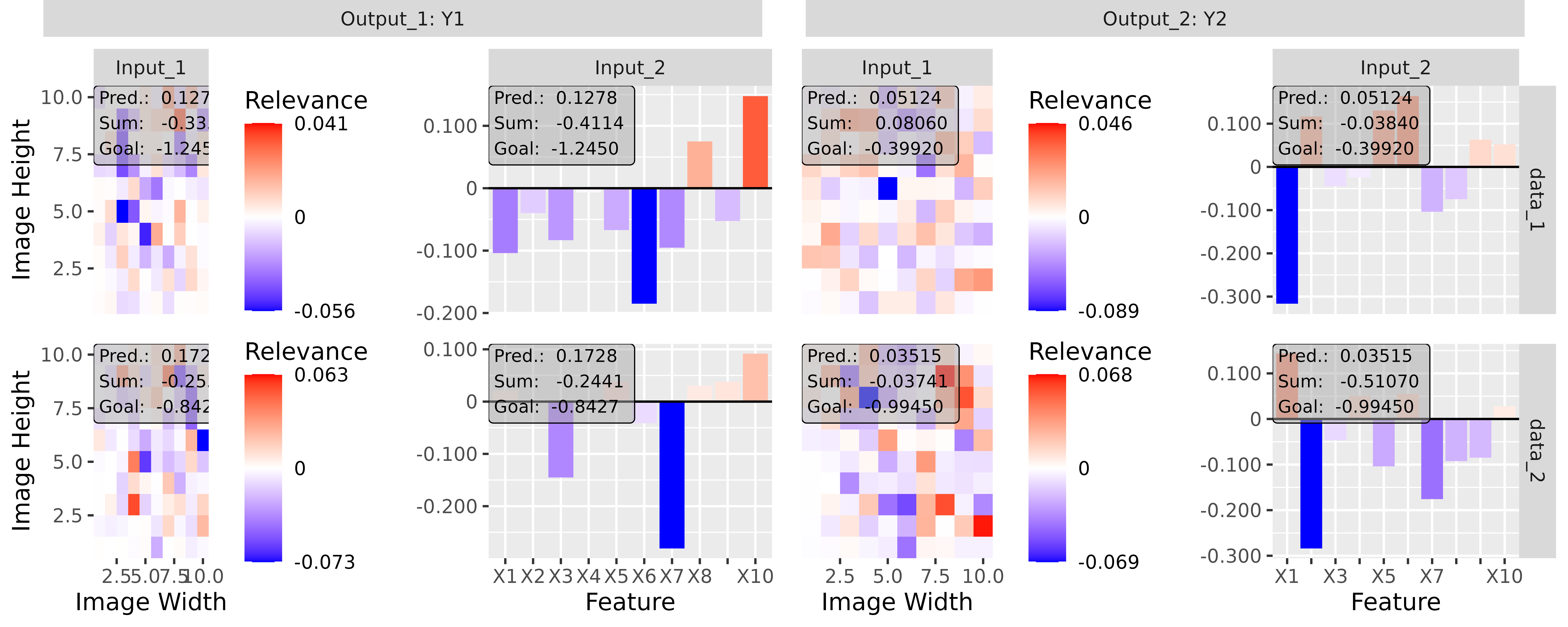
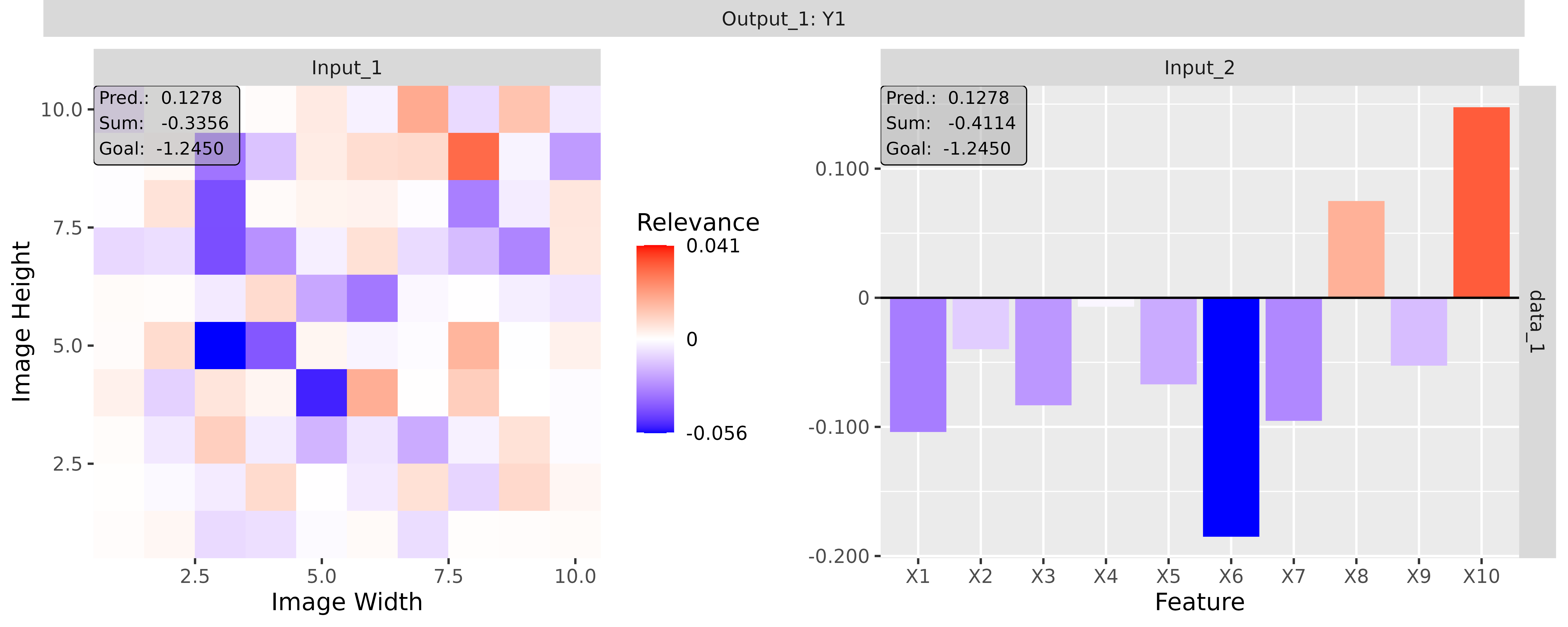
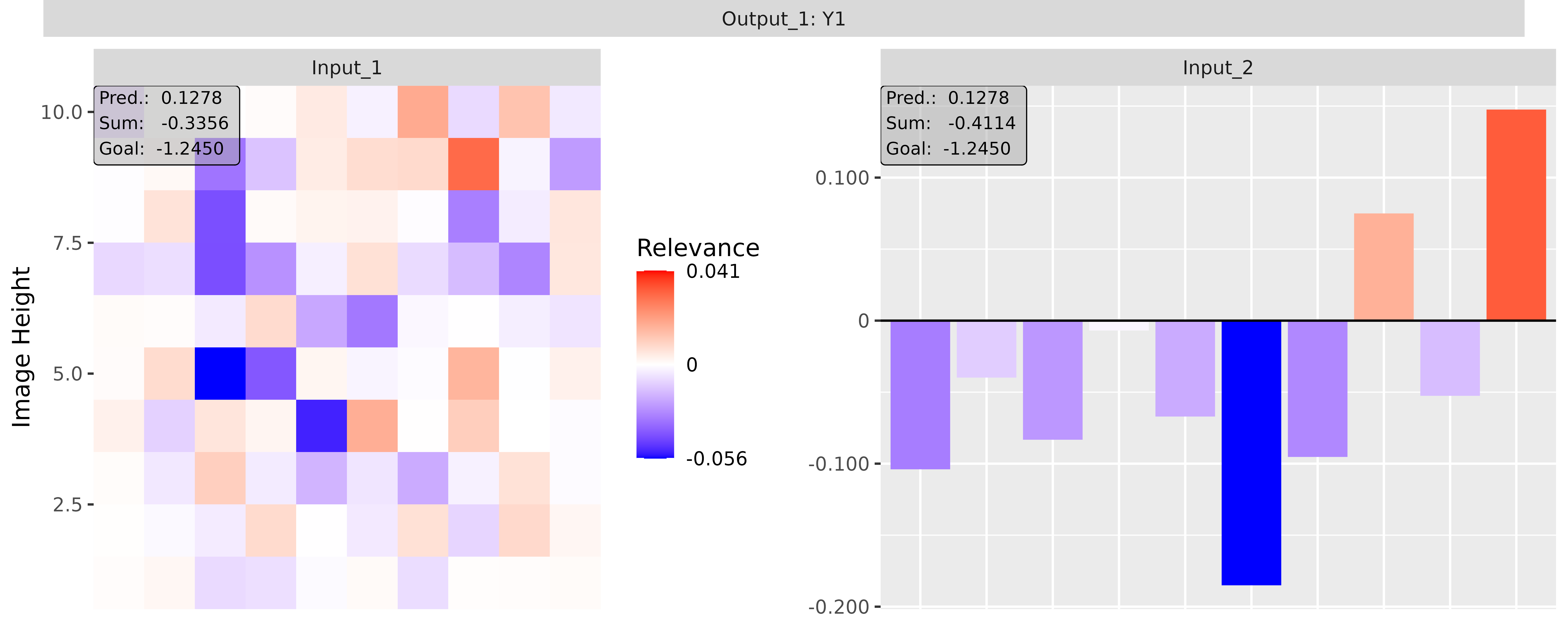
Plots based on plotly

As explained in the previous sections of Step 3, for each plot method, the argument as_plotly can be used to generate an interactive plot, which allows for more detailed analysis, especially for extensive models and results. However, these are created with the suggested package plotly, which should be installed in the R environment.
Analogous to the S4 class innsight_ggplot2, the class innsight_plotly is a simple extension of the library plotly instead of ggplot2. In this case, however, no distinction is made between a plot with multiple input or output layers except from additional strips. Hence, visualization can always be created in the same way:

1. The corresponding shapes and annotations of the slots shapes and annotations are added to each plot in plots. This also adds the strips for the output node (or input layer) at the top and, if necessary, the strips on the right side for the data points.

2. Subsequently, all individual plots are combined into a single plot object with the help of the function plotly::subplot (see ?plotly::subplot for details).

3. Lastly, the global elements from the layout slot are added and if there are multiple input layers (multiplot = TRUE), another output strip is added for the columns.

An example structure of the plot with multiple input layers is shown below:

|      Output 1: Node 1      |      Output 1: Node 3      |
|   Input 1   |   Input 2    |   Input 1   |   Input 2    |
|---------------------------------------------------------|-------------
|             |              |             |              |
| plots[1,1]  |  plots[1,2]  | plots[1,3]  | plots[1,4]   | data point 1
|             |              |             |              |
|---------------------------------------------------------|-------------
|             |              |             |              |
| plots[2,1]  |  plots[2,2]  | plots[2,3]  | plots[2,4]   | data point 2
| 

📝 Notes

• The plotly package is not a required package for innsight, so when creating interactive plotly-based plots, users should have it installed in their R environment on their own.

• The slots already mentioned and explained below, are for internal use only and generally should not be touched by users applying standard use cases.

• Due to the size of interactive plots, the following plotly-based plots are only rendered in the vignette at the pkdown website and not in the base R vignette!

Slots:

• plots : The individual plotly objects arranged as a matrix of size $(N_\text{datapoints}, N_\text{outputnodes} \cdot N_\text{inputlayers})$*.

• shapes : A list of two lists with the names shapes_strips and shapes_other. The list shapes_strips contains the shapes for the strips and may not be manipulated. The other list shapes_other contains a matrix of the same size as plots and each entry contains the shapes of the corresponding plot. For more details to shapes in plotly, we refer to the plotly website.

• annotations : A list of two lists with the names annotations_strips and annotations_other. The list annotations_strips contains the annotations for the strips and may not be manipulated. The other list annotations_other contains a matrix of the same size as plots and each entry contains the annotations of the corresponding plot. For more details to annotations in plotly, see ?plotly::add_annotations or the plotly website.

• multiplot : A logical value that indicates whether there are multiple input layers and thus whether another layer of strips should be created at the top of the plot.

• layout : This list contains all global layout options, e.g., update buttons, sliders, margins etc. (see ?plotly::layout for more details).

• col_dims : A list of two lists assigning a column index (col_idx) the corresponding output strip label (col_label).

# Create a plot for output node 1 in the first layer and output node 2 in the
# second layer and data point 1 and 3
p <- plot(res_two_inputs,
  output_idx = list(1, 2), data_idx = c(1, 3),
  as_plotly = TRUE
)

# Slot 'plots' is a 2x4 matrix (2 data points, 2 output nodes and 2 input layers)
p@plots
#>      [,1]     [,2]     [,3]     [,4]    
#> [1,] plotly,8 plotly,8 plotly,8 plotly,8
#> [2,] plotly,8 plotly,8 plotly,8 plotly,8

# Slot 'shapes' contains two 2x4 matrices with the corresponding shape objects
p@shapes
#> $shapes_strips
#>      [,1]   [,2]   [,3]   [,4]  
#> [1,] list,1 list,1 list,1 list,2
#> [2,] NULL   NULL   NULL   list,1
#> 
#> $shapes_other
#>      [,1] [,2]   [,3] [,4]  
#> [1,] NULL list,1 NULL list,1
#> [2,] NULL list,1 NULL list,1

# The same for the annotations
p@annotations
#> $annotations_strips
#>      [,1]   [,2]   [,3]   [,4]  
#> [1,] list,1 list,1 list,1 list,2
#> [2,] NULL   NULL   NULL   list,1
#> 
#> $annotations_other
#>      [,1] [,2] [,3] [,4]
#> [1,] NULL NULL NULL NULL
#> [2,] NULL NULL NULL NULL

# The model has multiple input layers, so the slot 'multiplot' is TRUE
p@multiplot
#> [1] TRUE

# The overall layout is stored in the slot 'layout'
str(p@layout, max.level = 1)
#> List of 5
#>  $ margin     :List of 2
#>  $ showlegend : logi FALSE
#>  $ updatemenus:List of 2
#>  $ annotations:List of 2
#>  $ sliders    : list()

# 'col_dims' assigns the label of the additional strips to the respective column
p@col_dims
#> $col_idx
#> [1] 1 1 2 2
#> 
#> $col_label
#> [1] "Output_1: Y1" "Output_2: Y2"

As described earlier, this S4 class generates a plotly object created by plotly::subplot, which can be treated and modified according to the syntax of the plotly package. Additionally, some generic functions are implemented to visualize individual aspects of the overall plot or to examine them in more detail. All available generic functions are listed below:

• [ : With this basic generic indexing function, the plots of individual rows and columns can be accessed and is returned as an object of the class innsight_plotly.

  Example

  # Create plot
  p <- plot(res_two_inputs,
    output_idx = list(1, 2), data_idx = c(1, 3),
    as_plotly = TRUE
  )
  
  # Show the whole plot
  p

  # Now you can select specific rows and columns for in-depth investigation,
  # e.g. only the result for output "Y2"
  p_new <- p[1:2, 3:4]
  
  # It's still an object of class 'innsight_plotly'
  class(p_new)
  #> [1] "innsight_plotly"
  #> attr(,"package")
  #> [1] "innsight"
  
  # Show the subplot
  p_new

• [[ : With this basic generic indexing function, you can select a single plot by passing the respective row and column index. This plot is returned as a plotly object.

  Example

  # Create plot
  p <- plot(res_two_inputs,
    output_idx = list(1, 2), data_idx = c(1, 3),
    as_plotly = TRUE
  )
  
  # Now you can select a single plot by passing the row and column index,
  # e.g. the plot for output "Y1", data point 3 and the second input layer
  p_new <- p[[2, 2]]
  
  # It's a plotly object
  class(p_new)
  #> [1] "plotly"     "htmlwidget"
  
  # Show the plot
  p_new
• plot, print and show : These methods provide generic visualization functions, which all behave the same in this case. They create the plot of the results and return a plotly object invisibly. For plot and print, you can also pass additional arguments forwarded to plotly::subplot.
  Examples

  # Create plot
  p <- plot(res_two_inputs,
    output_idx = list(1, 2), data_idx = 1,
    as_plotly = TRUE
  )
  
  # All methods behave the same and return a plotly object
  class(print(p))
  #> [1] "plotly"     "htmlwidget"
  class(show(p))
  #> [1] "plotly"     "htmlwidget"
  class(plot(p))
  #> [1] "plotly"     "htmlwidget"
  #>
  # You can also pass additional arguments to the method 'plotly::subplot',
  # e.g. the margins
  print(p, margin = c(0.03, 0.03, 0.01, 0.01))