Example 3: ImageNet with keras

This is a rather short article, just to illustrate the use of the innsight package on a few images of the ImageNet dataset and pre-trained keras models. For more detailed information about the package and the implemented methods we refer to this article and for simpler but in detailed explained examples we kindly recommend to Example 1 and Example 2.

In this example, we want to apply the innsight package on pre-trained models on the ImageNet dataset using keras. This dataset is a classification problem of images in $1000$ classes containing over $500$ images per class. We have selected examples of a few classes each and will analyze them with respect to different networks in the following.

Preprocess images

The original images all have different sizes and the pre-trained models all require an input size of $224 \times 224 \times 3$ and the channels are zero-centered according to the channel mean of the whole dataset; hence, we need to pre-process the images accordingly, which we will do in the following steps:

# Load required packages
library(keras)
library(innsight)

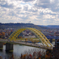
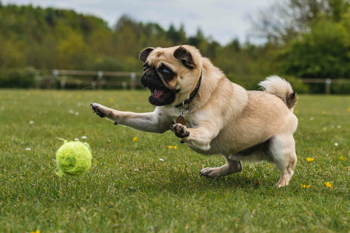
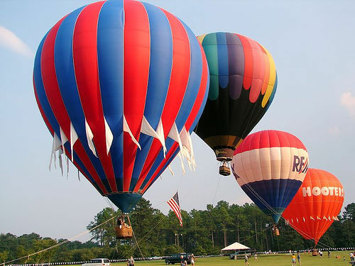
# Load images
img_files <- paste0("images/", c("image_1.png", "image_2.png", "image_3.png", "image_4.png"))
images <- k_stack(lapply(img_files, 
                 function(path) image_to_array(image_load(path, target_size = c(224, 224)))))

# now 'images' is a batch of 4 images of equal size 224x224x3
dim(images)
#> [1]   4 224 224   3

# preprocess images matching the conditions of the pre-trained models
images <- imagenet_preprocess_input(images)

Method configuration

Besides the images, we also need the labels of the $1000$ classes, which we get via a trick with the imagenet_decode_predictions() function:

# get class labels
res <- imagenet_decode_predictions(array(1:1000, dim = c(1,1000)), top = 1000)[[1]]
#> Downloading data from https://storage.googleapis.com/download.tensorflow.org/data/imagenet_class_index.json
#>  8192/35363 [=====>........................] - ETA: 0s35363/35363 [==============================] - 0s 0us/step
imagenet_labels <- res$class_description[order(res$class_name)]

Last but not least, we define the configurations for the methods we want to apply to the images and the models. This is a list that contains the method call, method name and the corresponding method arguments. For more information to the methods and the method-specific arguments, we refer to the in-depth vignette.

config <- list(
  list(
    method = Gradient$new, 
    method_name = "Gradient", 
    method_args = list()),
  list(
    method = SmoothGrad$new, 
    method_name = "SmoothGrad", 
    method_args = list(n = 10)),
  list(
    method = Gradient$new, 
    method_name = "Gradient x Input", 
    method_args = list(times_input = TRUE)),
  list(
    method = LRP$new, 
    method_name = "LRP (alpha_beta)", 
    method_args = list(
      rule_name = list(BatchNorm_Layer = "pass", Conv2D_Layer = "alpha_beta", 
                       MaxPool2D_Layer = "alpha_beta", Dense_Layer = "alpha_beta",
                       AvgPool2D_Layer = "alpha_beta"), 
      rule_param = 1)),
  list(
    method = LRP$new, 
    method_name = "LRP (composite)", 
    method_args = list(
      rule_name = list(BatchNorm_Layer = "pass", Conv2D_Layer = "alpha_beta", 
                       MaxPool2D_Layer = "epsilon", AvgPool2D_Layer = "alpha_beta"), 
      rule_param = list(Conv2D_Layer = 0.5, AvgPool2D_Layer = 0.5, 
                        MaxPool2D_Layer = 0.001))),
  list(
    method = DeepLift$new, 
    method_name = "DeepLift (rescale zeros)", 
    method_args = list()),
  list(
    method = DeepLift$new, 
    method_name = "DeepLift (reveal-cancel mean)",
    method_args = list(rule_name = "reveal_cancel", x_ref = "mean"))
)

In order to keep this article clear, we define a few utility functions below, which will be used later on.

Utility functions

# Function for getting the method arguments
get_method_args <- function(conf, converter, data, output_idx) {
  args <- conf$method_args
  args$converter <- converter
  args$data <- data 
  args$output_idx <- output_idx
  args$channels_first <- FALSE
  args$verbose <- FALSE
  
  # for DeepLift use the channel mean
  if (!is.null(args$x_ref)) {
    mean <- array(apply(as.array(args$data), c(1, 4), mean), dim = c(1,1,1,3))
    sd <- array(apply(as.array(args$data), c(1, 4), sd), dim = c(1,1,1,3))
    args$x_ref <- torch::torch_randn(c(1,224,224,3)) * sd + mean
  }
  
  args
}

apply_innsight <- function(method_conf, pred_df, FUN) {
  lapply(seq_len(nrow(pred_df)), # For each image...
       function(i) {
         do.call(rbind, args = lapply(method_conf, FUN, i = i)) # and each method...
       })
}

add_original_images <- function(img_files, gg_plot, num_methods) {
  library(png)
  
  img_pngs <- lapply(img_files, 
                 function(path) image_to_array(image_load(path, target_size = c(224, 224))) / 255)
  
  gl <- lapply(img_pngs, grid::rasterGrob)
  gl <- append(gl, list(gg_plot))
  
  num_images <- length(img_files)
  layout_matrix <- matrix(c(seq_len(num_images), 
                            rep(num_images + 1, num_images * num_methods)), 
                          nrow = num_images)
  
  list(grobs = gl, layout_matrix = layout_matrix)
}

Pre-trained model VGG19

Now let’s analyze the individual images according to the class that the model VGG19 (see ?application_vgg19 for details) predicts for them. In the innsight package, these output classes have to be chosen by ourselves because a calculation for all $1000$ classes would be too computationally expensive. For this reason, we first determine the corresponding predictions from the model:

# Load the model
model <- application_vgg19(include_top = TRUE, weights = "imagenet") 
#> Downloading data from https://storage.googleapis.com/tensorflow/keras-applications/vgg19/vgg19_weights_tf_dim_ordering_tf_kernels.h5
#>      8192/574710816 [..............................] - ETA: 0s  4202496/574710816 [..............................] - ETA: 15s 15310848/574710816 [..............................] - ETA: 6s  28925952/574710816 [>.............................] - ETA: 4s 42868736/574710816 [=>............................] - ETA: 3s 50339840/574710816 [=>............................] - ETA: 4s 63881216/574710816 [==>...........................] - ETA: 3s 76693504/574710816 [===>..........................] - ETA: 3s 90669056/574710816 [===>..........................] - ETA: 3s104693760/574710816 [====>.........................] - ETA: 2s109133824/574710816 [====>.........................] - ETA: 2s123248640/574710816 [=====>........................] - ETA: 2s135684096/574710816 [======>.......................] - ETA: 2s147546112/574710816 [======>.......................] - ETA: 2s159170560/574710816 [=======>......................] - ETA: 2s170737664/574710816 [=======>......................] - ETA: 2s182771712/574710816 [========>.....................] - ETA: 2s194600960/574710816 [=========>....................] - ETA: 2s206807040/574710816 [=========>....................] - ETA: 1s219062272/574710816 [==========>...................] - ETA: 1s231235584/574710816 [===========>..................] - ETA: 1s242778112/574710816 [===========>..................] - ETA: 1s254369792/574710816 [============>.................] - ETA: 1s266182656/574710816 [============>.................] - ETA: 1s272261120/574710816 [=============>................] - ETA: 1s284180480/574710816 [=============>................] - ETA: 1s297254912/574710816 [==============>...............] - ETA: 1s310476800/574710816 [===============>..............] - ETA: 1s323641344/574710816 [===============>..............] - ETA: 1s337240064/574710816 [================>.............] - ETA: 1s350388224/574710816 [=================>............] - ETA: 1s363732992/574710816 [=================>............] - ETA: 1s378101760/574710816 [==================>...........] - ETA: 0s391241728/574710816 [===================>..........] - ETA: 0s405061632/574710816 [====================>.........] - ETA: 0s418234368/574710816 [====================>.........] - ETA: 0s431988736/574710816 [=====================>........] - ETA: 0s445218816/574710816 [======================>.......] - ETA: 0s448438272/574710816 [======================>.......] - ETA: 0s458563584/574710816 [======================>.......] - ETA: 0s468688896/574710816 [=======================>......] - ETA: 0s482123776/574710816 [========================>.....] - ETA: 0s495206400/574710816 [========================>.....] - ETA: 0s508510208/574710816 [=========================>....] - ETA: 0s521674752/574710816 [==========================>...] - ETA: 0s535552000/574710816 [==========================>...] - ETA: 0s545267712/574710816 [===========================>..] - ETA: 0s560726016/574710816 [============================>.] - ETA: 0s574710816/574710816 [==============================] - 3s 0us/step

# get predictions
pred <- predict(model, images)
#> 1/1 - 1s - 1s/epoch - 1s/step
pred_df <- imagenet_decode_predictions(pred, top = 1)

# store the top prediction with the class label in a data.frame
pred_df <- do.call(rbind, args = lapply(pred_df, function(x) x[1, ]))

# add the model output index as a column
pred_df <- cbind(pred_df, index = apply(pred, 1, which.max))

# show the summary of the output predictions
pred_df
#>   class_name class_description     score index
#> 1  n04311004 steel_arch_bridge 0.7572441   822
#> 2  n02108422      bull_mastiff 0.4107325   244
#> 3  n11939491             daisy 0.2913898   986
#> 4  n02782093           balloon 0.9997583   418

Afterward, we apply all the methods from the configuration config to the model by first putting it into a Converter object and then applying the methods to each image individually.

# Step 1: Convert the model ----------------------------------------------------
converter <- Converter$new(model, output_names = imagenet_labels)

FUN <- function(conf, i) {
   # Get method args and add the converter, data, output index
   # channels first and verbose arguments
   args <- get_method_args(conf, converter, images[i,,,, drop = FALSE],  
                           pred_df$index[i])
   
   # Step 2: Apply method ------------------------------------------------------
   method <- do.call(conf$method, args = args)
   
   # Step 3: Get the result as a data.frame ------------------------------------
   result <- get_result(method, "data.frame")
   result$data <- paste0("data_", i)
   result$method <- conf$method_name
   
   # Tidy a bit..
   rm(method)
   gc()
   
   result
}

result <- apply_innsight(config, pred_df, FUN)

# Combine results and transform into data.table
library(data.table)
result <- data.table(do.call(rbind, result))

After the results have been generated and summarized in a data.table, they can be visualized using ggplot2:

library(ggplot2)

# First, we take the channels mean
result <- result[, .(value = mean(value)), 
                 by = c("data", "feature", "feature_2", "output_node", "method")]

# Now, we normalize the relevance values for each output, data point and method to [-1, 1]
result <- result[, .(value = value / max(abs(value)), feature = feature, feature_2 = feature_2),
                 by = c("data", "output_node", "method")]

result$method <- factor(result$method, levels = unique(result$method))

# set probabilities
labels <- paste0(pred_df$class_description, " (", round(pred_df$score * 100, 2), "%)")
result$data <- factor(result$data, levels = unique(result$data), labels = labels)

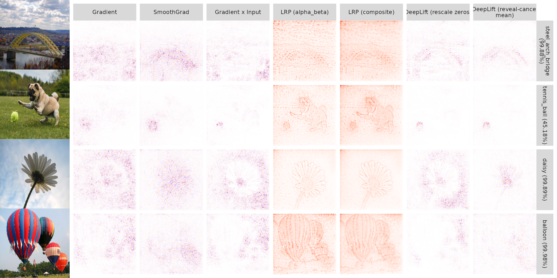
# Create ggplot2 plot
p <- ggplot(result) + 
  geom_raster(aes(x = as.numeric(feature_2), y = as.numeric(feature), fill= value)) +
  scale_fill_gradient2(guide = "none", mid = "white", low = "blue", high = "red") +
  facet_grid(rows = vars(data), cols = vars(method), 
             labeller = labeller(data = label_wrap_gen(), method = label_wrap_gen())) +
  scale_y_reverse(expand = c(0,0), breaks = NULL) + 
  scale_x_continuous(expand = c(0,0), breaks = NULL) +
  labs(x = NULL, y = NULL)


# Create column with the original images and show the combined plot
res <- add_original_images(img_files, p, length(unique(result$method)))
gridExtra::grid.arrange(grobs = res$grobs, layout_matrix = res$layout_matrix)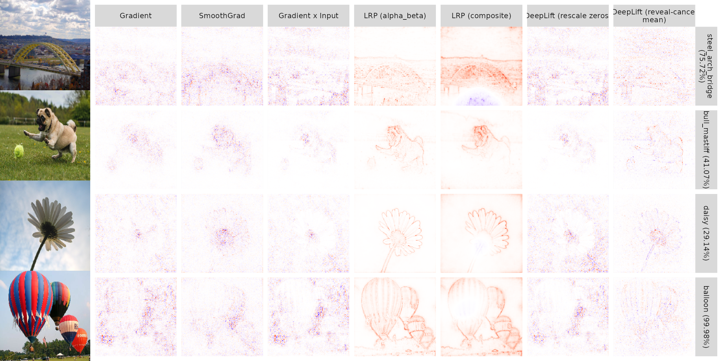

Pre-trained model ResNet50

We can execute these steps to another model analogously:

The exact same steps as in the last section

Load the model ResNet50 (see ?application_resnet50 for details) and get the predictions:

# Load the model
model <- application_resnet50(include_top = TRUE, weights = "imagenet") 
#> Downloading data from https://storage.googleapis.com/tensorflow/keras-applications/resnet/resnet50_weights_tf_dim_ordering_tf_kernels.h5
#>      8192/102967424 [..............................] - ETA: 0s  4202496/102967424 [>.............................] - ETA: 1s 17276928/102967424 [====>.........................] - ETA: 0s 34955264/102967424 [=========>....................] - ETA: 0s 52740096/102967424 [==============>...............] - ETA: 0s 70828032/102967424 [===================>..........] - ETA: 0s 83894272/102967424 [=======================>......] - ETA: 0s 95977472/102967424 [==========================>...] - ETA: 0s102967424/102967424 [==============================] - 0s 0us/step

# get predictions
pred <- predict(model, images)
#> 1/1 - 1s - 932ms/epoch - 932ms/step
pred_df <- imagenet_decode_predictions(pred, top = 1)

# store the top prediction with the class label in a data.frame
pred_df <- do.call(rbind, args = lapply(pred_df, function(x) x[1, ]))

# add the model output index as a column
pred_df <- cbind(pred_df, index = apply(pred, 1, which.max))

Apply all methods specified in config to all images:

# Step 1: Convert the model ----------------------------------------------------
converter <- Converter$new(model, output_names = imagenet_labels)

FUN <- function(conf, i) {
   # Get method args and add the converter, data, output index
   # channels first and verbose arguments
   args <- get_method_args(conf, converter, images[i,,,, drop = FALSE],  
                           pred_df$index[i])
   
   # Step 2: Apply method ------------------------------------------------------
   method <- do.call(conf$method, args = args)
   
   # Step 3: Get the result as a data.frame ------------------------------------
   result <- get_result(method, "data.frame")
   result$data <- paste0("data_", i)
   result$method <- conf$method_name
   
   # Tidy a bit..
   rm(method)
   gc()
   
   result
}

result <- apply_innsight(config, pred_df, FUN)

# Combine results and transform into data.table
library(data.table)
result <- data.table(do.call(rbind, result))

After the results have been generated and summarized in a data.table, they can be visualized using ggplot2:

library(ggplot2)

# First, we take the channels mean
result <- result[, .(value = mean(value)), 
                 by = c("data", "feature", "feature_2", "output_node", "method")]

# Now, we normalize the relevance values for each output, data point and method to [-1, 1]
result <- result[, .(value = value / max(abs(value)), feature = feature, feature_2 = feature_2),
                 by = c("data", "output_node", "method")]

result$method <- factor(result$method, levels = unique(result$method))

# set probabilities
labels <- paste0(pred_df$class_description, " (", round(pred_df$score * 100, 2), "%)")
result$data <- factor(result$data, levels = unique(result$data), labels = labels)

# Create ggplot2 plot
p <- ggplot(result) + 
  geom_raster(aes(x = as.numeric(feature_2), y = as.numeric(feature), fill= value)) +
  scale_fill_gradient2(guide = "none", mid = "white", low = "blue", high = "red") +
  facet_grid(rows = vars(data), cols = vars(method), 
             labeller = labeller(data = label_wrap_gen(), method = label_wrap_gen())) +
  scale_y_reverse(expand = c(0,0), breaks = NULL) + 
  scale_x_continuous(expand = c(0,0), breaks = NULL) +
  labs(x = NULL, y = NULL)


# Create column with the original images and show the combined plot

res <- add_original_images(img_files, p, length(unique(result$method)))

Show the result:

gridExtra::grid.arrange(grobs = res$grobs, layout_matrix = res$layout_matrix)