The Expected Gradients method (Erion et al., 2021), also known as
GradSHAP, is a local feature attribution technique which extends the
IntegratedGradient method and provides approximate Shapley values. In
contrast to IntegratedGradient, it considers not only a single reference
value \(x'\) but the whole distribution of reference values
\(X' \sim x'\) and averages the IntegratedGradient values over this
distribution. Mathematically, the method can be described as follows:
$$
E_{x'\sim X', \alpha \sim U(0,1)}[(x - x') \times \frac{\partial f(x' + \alpha (x - x'))}{\partial x}]
$$
The distribution of the reference values is specified with the argument
data_ref, of which n samples are taken at random for each instance
during the estimation.
The R6 class can also be initialized using the run_expgrad function
as a helper function so that no prior knowledge of R6 classes is required.
Direct torch alternative
For torch models, a lightweight alternative is available via
torch_expgrad that uses native torch autograd directly without
requiring the Converter step. Raw tensor results can be wrapped
into the standard innsight format using as_innsight_result.
References
G. Erion et al. (2021) *Improving performance of deep learning models with * axiomatic attribution priors and expected gradients. Nature Machine Intelligence 3, pp. 620-631.
See also
Other methods:
ConnectionWeights,
DeepLift,
DeepSHAP,
Gradient,
IntegratedGradient,
LIME,
LRP,
SHAP,
SmoothGrad
Super classes
innsight::InterpretingMethod -> innsight::GradientBased -> ExpectedGradient
Public fields
n(
integer(1))
Number of samples from the distribution of reference values and number of samples for the approximation of the integration path along \(\alpha\) (default: \(50\)).data_ref(
list)
The reference input for the ExpectedGradient method. This value is stored as a list oftorch_tensors of shape ( , dim_in) for each input layer.
Methods
Method new()
Create a new instance of the ExpectedGradient R6 class. When
initialized, the method Expected Gradient is applied to the given
data and baseline values and the results are stored in the field result.
Usage
ExpectedGradient$new(
  converter,
  data,
  data_ref = NULL,
  n = 50,
  channels_first = TRUE,
  output_idx = NULL,
  output_label = NULL,
  ignore_last_act = TRUE,
  verbose = interactive(),
  dtype = "float"
)
Arguments
converter(
Converter)
An instance of theConverterclass that includes the torch-converted model and some other model-specific attributes. SeeConverterfor details.data(
array,data.frame,torch_tensororlist)
The data to which the method is to be applied. These must have the same format as the input data of the passed model to the converter object. This means eitheran
array,data.frame,torch_tensoror array-like format of size (batch_size, dim_in), if e.g., the model has only one input layer, ora
listwith the corresponding input data (according to the upper point) for each of the input layers.
data_ref(
array,data.frame,torch_tensororlist)
The reference inputs for the ExpectedGradient method. This value must have the same format as the input data of the passed model to the converter object. This means eitheran
array,data.frame,torch_tensoror array-like format of size ( , dim_in), if e.g., the model has only one input layer, ora
listwith the corresponding input data (according to the upper point) for each of the input layers.It is also possible to use the default value
NULLto take only zeros as reference input.
n(
integer(1))
Number of samples from the distribution of reference values and number of samples for the approximation of the integration path along \(\alpha\) (default: \(50\)).channels_first(
logical(1))
The channel position of the given data (argumentdata). IfTRUE, the channel axis is placed at the second position between the batch size and the rest of the input axes, e.g.,c(10,3,32,32)for a batch of ten images with three channels and a height and width of 32 pixels. Otherwise (FALSE), the channel axis is at the last position, i.e.,c(10,32,32,3). If the data has no channel axis, use the default valueTRUE.output_idx(
integer,listorNULL)
These indices specify the output nodes for which the method is to be applied. In order to allow models with multiple output layers, there are the following possibilities to select the indices of the output nodes in the individual output layers:An
integervector of indices: If the model has only one output layer, the values correspond to the indices of the output nodes, e.g.,c(1,3,4)for the first, third and fourth output node. If there are multiple output layers, the indices of the output nodes from the first output layer are considered.A
listofintegervectors of indices: If the method is to be applied to output nodes from different layers, a list can be passed that specifies the desired indices of the output nodes for each output layer. Unwanted output layers have the entryNULLinstead of a vector of indices, e.g.,list(NULL, c(1,3))for the first and third output node in the second output layer.NULL(default): The method is applied to all output nodes in the first output layer but is limited to the first ten as the calculations become more computationally expensive for more output nodes.
output_label(
character,factor,listorNULL)
These values specify the output nodes for which the method is to be applied. Only values that were previously passed with the argumentoutput_namesin theconvertercan be used. In order to allow models with multiple output layers, there are the following possibilities to select the names of the output nodes in the individual output layers:A
charactervector orfactorof labels: If the model has only one output layer, the values correspond to the labels of the output nodes named in the passedConverterobject, e.g.,c("a", "c", "d")for the first, third and fourth output node if the output names arec("a", "b", "c", "d"). If there are multiple output layers, the names of the output nodes from the first output layer are considered.A
listofcharactor/factorvectors of labels: If the method is to be applied to output nodes from different layers, a list can be passed that specifies the desired labels of the output nodes for each output layer. Unwanted output layers have the entryNULLinstead of a vector of labels, e.g.,list(NULL, c("a", "c"))for the first and third output node in the second output layer.NULL(default): The method is applied to all output nodes in the first output layer but is limited to the first ten as the calculations become more computationally expensive for more output nodes.
ignore_last_act(
logical(1))
Set this logical value to include the last activation functions for each output layer, or not (default:TRUE). In practice, the last activation (especially for softmax activation) is often omitted.verbose(
logical(1))
This logical argument determines whether a progress bar is displayed for the calculation of the method or not. The default value is the output of the primitive R functioninteractive().dtype(
character(1))
The data type for the calculations. Use either'float'fortorch_floator'double'fortorch_double.
Examples
#----------------------- Example 1: Torch ----------------------------------
library(torch)
# Create nn_sequential model and data
model <- nn_sequential(
nn_linear(5, 12),
nn_relu(),
nn_linear(12, 2),
nn_softmax(dim = 2)
)
data <- torch_randn(25, 5)
ref <- torch_randn(1, 5)
# Create Converter
converter <- convert(model, input_dim = c(5))
# Apply method IntegratedGradient
int_grad <- IntegratedGradient$new(converter, data, x_ref = ref)
# You can also use the helper function `run_intgrad` for initializing
# an R6 IntegratedGradient object
int_grad <- run_intgrad(converter, data, x_ref = ref)
# Print the result as a torch tensor for first two data points
get_result(int_grad, "torch.tensor")[1:2]
#> torch_tensor
#> (1,.,.) =
#> -0.2239 -0.1661
#> -0.0402 -0.3057
#> 0.0613 0.1847
#> 0.1857 0.2844
#> 0.1127 0.1611
#>
#> (2,.,.) =
#> 0.0046 0.0043
#> -0.0097 0.0339
#> -0.0739 -0.0993
#> 0.4103 0.4057
#> 0.1486 0.1576
#> [ CPUFloatType{2,5,2} ]
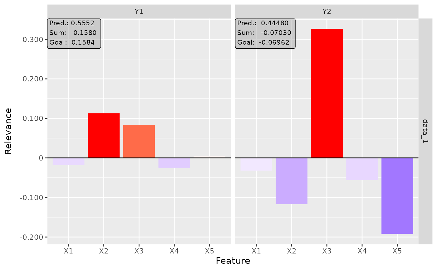
# Plot the result for both classes
plot(int_grad, output_idx = 1:2)
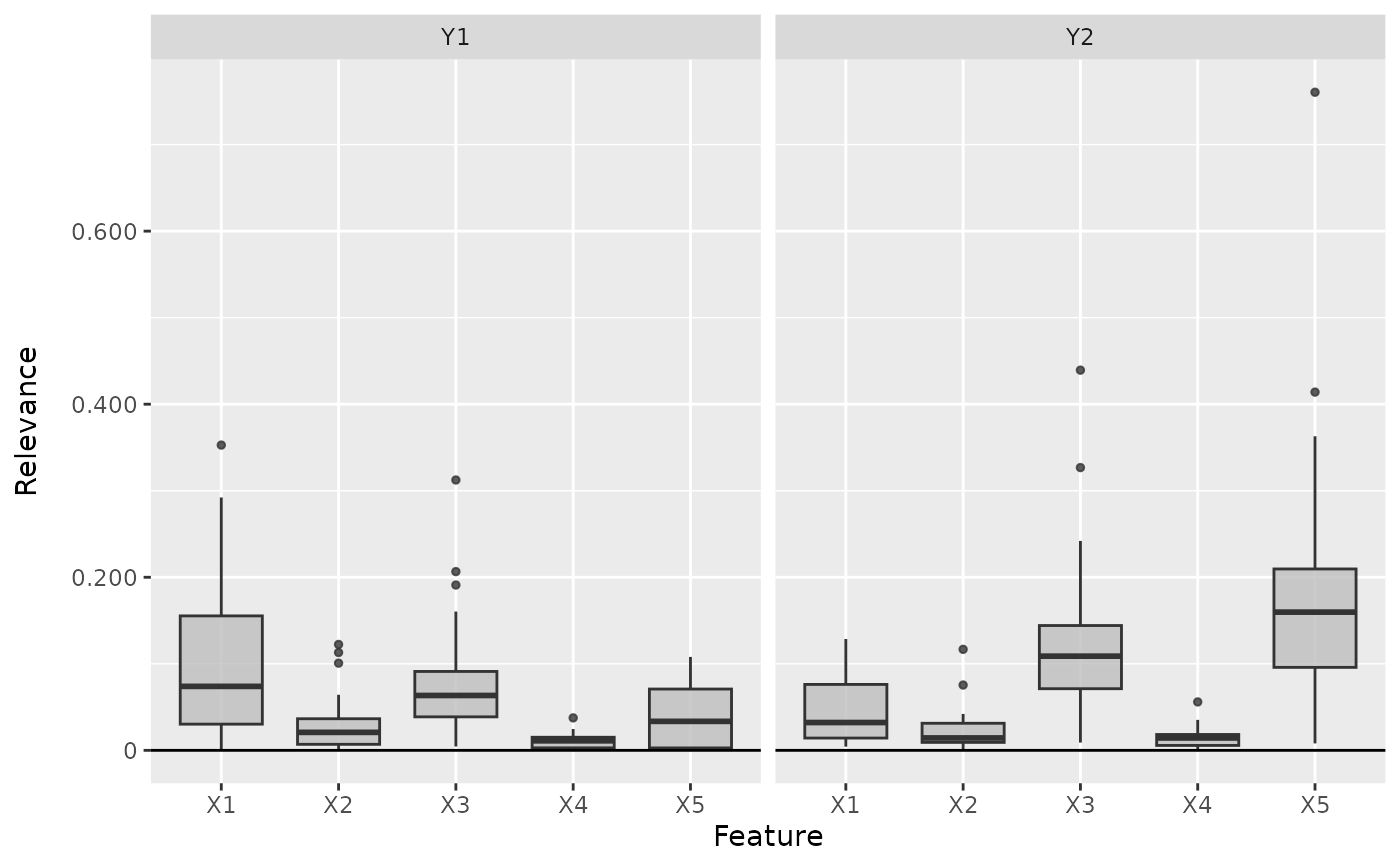
 # Plot the boxplot of all datapoints and for both classes
boxplot(int_grad, output_idx = 1:2)
# Plot the boxplot of all datapoints and for both classes
boxplot(int_grad, output_idx = 1:2)
 # ------------------------- Example 2: Neuralnet ---------------------------
if (require("neuralnet")) {
library(neuralnet)
data(iris)
# Train a neural network
nn <- neuralnet((Species == "setosa") ~ Petal.Length + Petal.Width,
iris,
linear.output = FALSE,
hidden = c(3, 2), act.fct = "tanh", rep = 1
)
# Convert the model
converter <- convert(nn)
# Apply IntegratedGradient with a reference input of the feature means
x_ref <- matrix(colMeans(iris[, c(3, 4)]), nrow = 1)
int_grad <- run_intgrad(converter, iris[, c(3, 4)], x_ref = x_ref)
# Get the result as a dataframe and show first 5 rows
get_result(int_grad, type = "data.frame")[1:5, ]
# Plot the result for the first datapoint in the data
plot(int_grad, data_idx = 1)
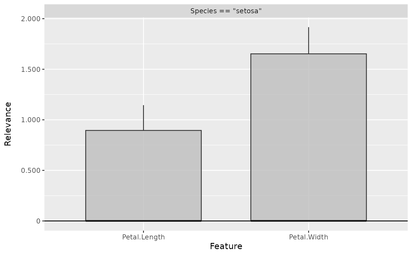
# Plot the result as boxplots
boxplot(int_grad)
}
# ------------------------- Example 2: Neuralnet ---------------------------
if (require("neuralnet")) {
library(neuralnet)
data(iris)
# Train a neural network
nn <- neuralnet((Species == "setosa") ~ Petal.Length + Petal.Width,
iris,
linear.output = FALSE,
hidden = c(3, 2), act.fct = "tanh", rep = 1
)
# Convert the model
converter <- convert(nn)
# Apply IntegratedGradient with a reference input of the feature means
x_ref <- matrix(colMeans(iris[, c(3, 4)]), nrow = 1)
int_grad <- run_intgrad(converter, iris[, c(3, 4)], x_ref = x_ref)
# Get the result as a dataframe and show first 5 rows
get_result(int_grad, type = "data.frame")[1:5, ]
# Plot the result for the first datapoint in the data
plot(int_grad, data_idx = 1)
# Plot the result as boxplots
boxplot(int_grad)
}
 # ------------------------- Example 3: Keras -------------------------------
if (require("keras") & keras::is_keras_available()) {
library(keras)
# Make sure keras is installed properly
is_keras_available()
data <- array(rnorm(10 * 32 * 32 * 3), dim = c(10, 32, 32, 3))
model <- keras_model_sequential()
model %>%
layer_conv_2d(
input_shape = c(32, 32, 3), kernel_size = 8, filters = 8,
activation = "softplus", padding = "valid") %>%
layer_conv_2d(
kernel_size = 8, filters = 4, activation = "tanh",
padding = "same") %>%
layer_conv_2d(
kernel_size = 4, filters = 2, activation = "relu",
padding = "valid") %>%
layer_flatten() %>%
layer_dense(units = 64, activation = "relu") %>%
layer_dense(units = 2, activation = "softmax")
# Convert the model
converter <- convert(model)
# Apply the IntegratedGradient method with a zero baseline and n = 20
# iteration steps
int_grad <- run_intgrad(converter, data,
channels_first = FALSE,
n = 20
)
# Plot the result for the first image and both classes
plot(int_grad, output_idx = 1:2)
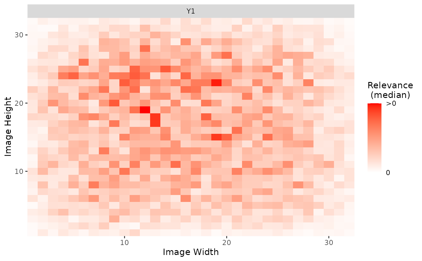
# Plot the pixel-wise median of the results
plot_global(int_grad, output_idx = 1)
}
# ------------------------- Example 3: Keras -------------------------------
if (require("keras") & keras::is_keras_available()) {
library(keras)
# Make sure keras is installed properly
is_keras_available()
data <- array(rnorm(10 * 32 * 32 * 3), dim = c(10, 32, 32, 3))
model <- keras_model_sequential()
model %>%
layer_conv_2d(
input_shape = c(32, 32, 3), kernel_size = 8, filters = 8,
activation = "softplus", padding = "valid") %>%
layer_conv_2d(
kernel_size = 8, filters = 4, activation = "tanh",
padding = "same") %>%
layer_conv_2d(
kernel_size = 4, filters = 2, activation = "relu",
padding = "valid") %>%
layer_flatten() %>%
layer_dense(units = 64, activation = "relu") %>%
layer_dense(units = 2, activation = "softmax")
# Convert the model
converter <- convert(model)
# Apply the IntegratedGradient method with a zero baseline and n = 20
# iteration steps
int_grad <- run_intgrad(converter, data,
channels_first = FALSE,
n = 20
)
# Plot the result for the first image and both classes
plot(int_grad, output_idx = 1:2)
# Plot the pixel-wise median of the results
plot_global(int_grad, output_idx = 1)
}
 #------------------------- Plotly plots ------------------------------------
if (require("plotly")) {
# You can also create an interactive plot with plotly.
# This is a suggested package, so make sure that it is installed
library(plotly)
boxplot(int_grad, as_plotly = TRUE)
}
#> Warning: The `boxplot()` function is only intended for tabular or signal data. It is
#> called `plot_global()` instead.
#------------------------- Plotly plots ------------------------------------
if (require("plotly")) {
# You can also create an interactive plot with plotly.
# This is a suggested package, so make sure that it is installed
library(plotly)
boxplot(int_grad, as_plotly = TRUE)
}
#> Warning: The `boxplot()` function is only intended for tabular or signal data. It is
#> called `plot_global()` instead.