library(mlr3verse) # All the mlr3 things
library(effectplots) # For effects plotting
lgr::get_logger("mlr3")$set_threshold("error")

# Penguin Task setup
penguins <- na.omit(palmerpenguins::penguins)
penguin_task <- as_task_classif(
  penguins,
  target = "species"
)Feature Importance
Goals of this part:
- Introduce (some) variable importance measures
- Compare measures for different settings
1 Feature Importance
Feature importance falls under the umbrella of interpretability, which is a huge topic, and there’s a lot to explore — we’ll cover some basics and if you’re interested, you can always find more at
- The IML lecture (free slides, videos)
- The Interpretable Machine Learning book
- The
{mlr3}book chapter
Before we get started with the general methods, it should be noted that some learners bring their own method-specific importance measures. Random Forests (via {ranger}) for example has some built-in importance metrics, like the corrected Gini impurity:
lrn_ranger <- lrn("classif.ranger", importance = "impurity_corrected")
lrn_ranger$train(penguin_task)

sort(lrn_ranger$importance(), decreasing = TRUE)
#> bill_length_mm flipper_length_mm bill_depth_mm island
#> 54.2401385 36.3183500 26.7463551 22.5503396
#> body_mass_g sex year
#> 21.5675075 0.8636880 -0.5303487Which shows us that for our penguins, bill_length_mm is probably the most relevant feature, whereas body_mass_g does not turn out to be as important with regard to species classification. THe year doesn’t seem to be useful for prediction at all — which is perfectly plausible!
1.1 Feature Importance with {mlr3filters}
The mlr3filters package provides some global, marginal importance methods, meaning they consider the relationship between the target and one feature at a time.
as.data.table(mlr_filters)[1:20, .(key, label)]#> Key: <key>
#> key label
#> <char> <char>
#> 1: anova ANOVA F-Test
#> 2: auc Area Under the ROC Curve Score
#> 3: boruta Burota
#> 4: carscore Correlation-Adjusted coRrelation Score
#> 5: carsurvscore Correlation-Adjusted coRrelation Survival Score
#> 6: cmim Minimal Conditional Mutual Information Maximization
#> 7: correlation Correlation
#> 8: disr Double Input Symmetrical Relevance
#> 9: find_correlation Correlation-based Score
#> 10: importance Importance Score
#> 11: information_gain Information Gain
#> 12: jmi Joint Mutual Information
#> 13: jmim Minimal Joint Mutual Information Maximization
#> 14: kruskal_test Kruskal-Wallis Test
#> 15: mim Mutual Information Maximization
#> 16: mrmr Minimum Redundancy Maximal Relevancy
#> 17: njmim Minimal Normalised Joint Mutual Information Maximization
#> 18: performance Predictive Performance
#> 19: permutation Permutation Score
#> 20: relief RELIEF
#> key labelOne “trick” of the filters package is that it can be used to access the $importance() that some learners provide on their own, and ranger provides the impurtiy-importance and permutation feature importance (PFI). We can access either with mlr3filters directly, but note it retrains the learner:
lrn_ranger <- lrn("classif.ranger", importance = "impurity_corrected")
filter_importance = flt("importance", learner = lrn_ranger)
filter_importance$calculate(penguin_task)

filter_importance
#> <FilterImportance:importance>: Importance Score
#> Task Types: classif
#> Properties: missings
#> Task Properties: -
#> Packages: mlr3, mlr3learners, ranger
#> Feature types: logical, integer, numeric, character, factor, ordered
#> feature score
#> 1: bill_length_mm 50.976878008
#> 2: flipper_length_mm 36.856975328
#> 3: bill_depth_mm 25.799481552
#> 4: body_mass_g 21.751449304
#> 5: island 20.717986260
#> 6: sex 0.848159529
#> 7: year -0.003874481mlr3filters also provides a general implementation for PFI that retrains the learner repeatedly with one feature randomly shuffled.
lrn_ranger <- lrn("classif.ranger")
filter_permutation = flt("permutation", learner = lrn_ranger)
filter_permutation$calculate(penguin_task)

filter_permutation
#> <FilterPermutation:permutation>: Permutation Score
#> Task Types: classif
#> Properties: missings
#> Task Properties: -
#> Packages: mlr3, mlr3learners, ranger, mlr3measures
#> Feature types: logical, integer, numeric, character, factor, ordered
#> feature score
#> 1: bill_length_mm 1.00000000
#> 2: bill_depth_mm 0.09626437
#> 3: island 0.09195402
#> 4: sex 0.08764368
#> 5: body_mass_g 0.06896552
#> 6: flipper_length_mm 0.04885057
#> 7: year 0.02442529But that also means we can use PFI for any other learner, such the SVM or XGBoost!
1.2 Your Turn!
- Compute PFI with
rangerusing it’s built-in$importance(), usingmlr3filters - Compute PFI for an SVM using the approproate
"permutation"filter - Comapre the two methods. Do they agree?
# Your code
mlr3 preprocessing pipelines
Note that we need to use the encoding PipeOp to train the SVM of these on the penguins task, as they can’t handle categorical features automatically:
lrn_svm <- po("encode") %>>%
  po("learner", lrn("classif.svm", kernel = "radial", <any other parameter>)) |>
  as_learner()
Example solution
This is just for demonstration — we’d need to use tuned hyperparameters for the SVM for a proper comparison!
penguin_task <- as_task_classif(
  na.omit(palmerpenguins::penguins),
  target = "species"
)

lrn_svm <- po("encode") %>>%
  po("learner", lrn("classif.svm")) |>
  as_learner()

pfi_svm = flt("permutation", learner = lrn_svm)
pfi_svm$calculate(penguin_task)
pfi_svm
#> <FilterPermutation:permutation>: Permutation Score
#> Task Types: classif
#> Properties: missings
#> Task Properties: -
#> Packages: mlr3, mlr3pipelines, stats, mlr3learners, e1071, mlr3measures
#> Feature types: logical, integer, numeric, character, factor, ordered,
#> POSIXct, Date
#> feature score
#> 1: bill_length_mm 1.00000000
#> 2: island -0.03846154
#> 3: bill_depth_mm -0.07122507
#> 4: sex -0.07122507
#> 5: flipper_length_mm -0.08974359
#> 6: body_mass_g -0.09116809
#> 7: year -0.10113960pfi_ranger = flt("importance", learner = lrn("classif.ranger", importance = "permutation"))
pfi_ranger$calculate(penguin_task)
pfi_ranger#> <FilterImportance:importance>: Importance Score
#> Task Types: classif
#> Properties: missings
#> Task Properties: -
#> Packages: mlr3, mlr3learners, ranger
#> Feature types: logical, integer, numeric, character, factor, ordered
#> feature score
#> 1: bill_length_mm 0.2502032220
#> 2: flipper_length_mm 0.1517506849
#> 3: bill_depth_mm 0.1254753264
#> 4: island 0.1247705530
#> 5: body_mass_g 0.0887346455
#> 6: sex 0.0130695250
#> 7: year -0.00025549211.3 Feature Effects with {effectplots}
Getting a number for “is this feature important” is nice, but often we want a better picture of the feature’s effect. Think of linear models and how we can interpret \(\beta_j\) as the linear relationship between \(X_j\) and \(Y\) — often things aren’t linear though.
One approach to visualize feature effects is via Partial Dependence Plots or preferably via Accumulated Local Effect plots (ALE), which we get from the {effectplots} thankfully offers.
Let’s recycle our ranger learner and plot some effects, using the partial dependence plot (PDP) as an example:
lrn_ranger_cl <- lrn("classif.ranger", predict_type = "prob")
lrn_ranger_cl$train(penguin_task)

pd_penguins <- partial_dependence(
  object = lrn_ranger_cl$model,
  v = penguin_task$feature_names,
  data = penguin_task$data(),
  which_pred = "Adelie"
)

plot(pd_penguins)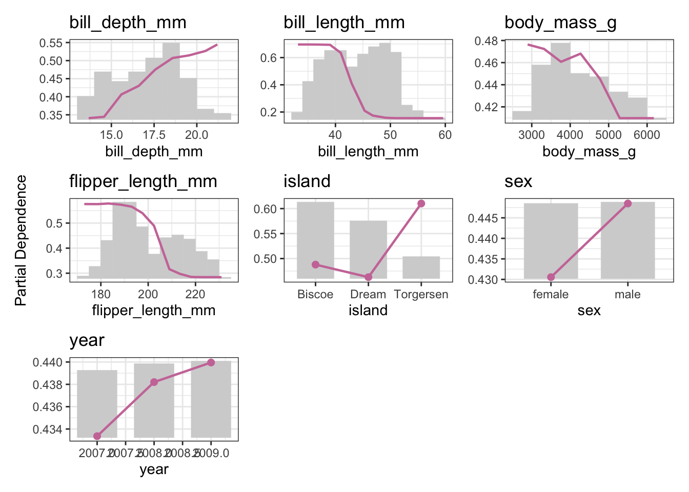
Note
We’re doing multiclass classification here, so while our learner predicts a probability for one of each of the three target classes (Adelie, Gentoo, Chinstrap), we need to pick one for the visualization!
1.4 Your turn! (Possibly for another time)
- Use the
bike_shareregression task to calculate the PDP - Stick with the
rangerlearner as{effectplots}supports it directly.
# your code
Example solution
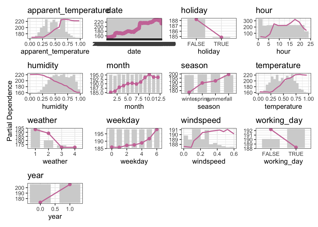
The bike_sharing task is a regression task, so make sure to switch to the regression version of the learner.
The target is bikers, the number of people using a specific bike sharing service. More information can be found on the UCI website.
task <- tsk("bike_sharing")
lrn_ranger <- lrn("regr.ranger")
lrn_ranger$train(task)

pd_bikeshare <- partial_dependence(
  object = lrn_ranger$model,
  v = task$feature_names,
  data = task$data()
)

plot(pd_bikeshare)