library(ggplot2) # For plotting
library(palmerpenguins) # For penguins
library(mlr3verse) # includes mlr3, mlr3learners, mlr3tuning, mlr3viz, ...Introducing {mlr3}
Goals of this part:
- Introduce
{mlr3}and do everythign we did before again, but nicer
1 Switching to {mlr3}
Now, imagine you want to try out some more hyperparameters for either rpart() or kknn() or both, and then you want to compare the two — that would probably be kind of tedious unless you write some wrapper functions, right? Well, luckily we’re not the first people to do some machine learning!
Our code in the previous section works (hopefully), but for any given model or algorithm, there’s different R packages with slightly different interfaces, and memorizing or looking up how they work can be a tedious and error-prone task, especially when we want to repeat the same general steps with each learner. {mlr3} and add-on packages unify all the common tasks with a consistent interface.
1.1 Creating a task
The task encapsulates our data, including which features we’re using for learning and wich variable we use as the target for prediction. Tasks can be created in multiple ways and some standard example tasks are available in mlr3, but we’re taking the long way around.
Questions a task object answers:
- What is the task type, what kind of prediction are we doing?
- Here: Classification (instead of e.g. regression)
- What are we predicting on?
- The dataset (“backend”), could be a
data.frame,matrix, or a proper data base
- The dataset (“backend”), could be a
- What variable are we trying to predict?
- The
targetvariable, herespecies
- The
- Which variables are we using for predictions?
- The
featurevariables, which we can adjust
- The
So let’s put our penguins into a task object for {mlr3} and inspect it:
# Creating a classification task from our penguin data
penguin_task <- as_task_classif(
  na.omit(palmerpenguins::penguins),
  id = "penguins",
  target = "species"
)

penguin_task
#>
#> ── <TaskClassif> (333x8) ───────────────────────────────────────────────────────
#> • Target: species
#> • Target classes: Adelie (44%), Gentoo (36%), Chinstrap (20%)
#> • Properties: multiclass
#> • Features (7):
#> • int (3): body_mass_g, flipper_length_mm, year
#> • dbl (2): bill_depth_mm, bill_length_mm
#> • fct (2): island, sexWe can poke at it a little. Try typing penguin_task$ and hit the Tab key to trigger completions.
# Contains our penguin dataset
penguin_task$data()
#> species bill_depth_mm bill_length_mm body_mass_g flipper_length_mm
#> <fctr> <num> <num> <int> <int>
#> 1: Adelie 18.7 39.1 3750 181
#> 2: Adelie 17.4 39.5 3800 186
#> 3: Adelie 18.0 40.3 3250 195
#> 4: Adelie 19.3 36.7 3450 193
#> 5: Adelie 20.6 39.3 3650 190
#> ---
#> 329: Chinstrap 19.8 55.8 4000 207
#> 330: Chinstrap 18.1 43.5 3400 202
#> 331: Chinstrap 18.2 49.6 3775 193
#> 332: Chinstrap 19.0 50.8 4100 210
#> 333: Chinstrap 18.7 50.2 3775 198
#> island sex year
#> <fctr> <fctr> <int>
#> 1: Torgersen male 2007
#> 2: Torgersen female 2007
#> 3: Torgersen female 2007
#> 4: Torgersen female 2007
#> 5: Torgersen male 2007
#> ---
#> 329: Dream male 2009
#> 330: Dream female 2009
#> 331: Dream male 2009
#> 332: Dream male 2009
#> 333: Dream female 2009# We can ask it about e.g. our sample size and number of features
penguin_task$nrow#> [1] 333penguin_task$ncol#> [1] 8# And what the classes are
penguin_task$class_names#> [1] "Adelie" "Chinstrap" "Gentoo"# What types of features do we have?
# (relevant for learner support, some don't handle factors for example!)
penguin_task$feature_types#> Key: <id>
#> id type
#> <char> <char>
#> 1: bill_depth_mm numeric
#> 2: bill_length_mm numeric
#> 3: body_mass_g integer
#> 4: flipper_length_mm integer
#> 5: island factor
#> 6: sex factor
#> 7: year integerWe can further inspect and modify the task after the fact if we choose:
# Display feature and target variable assignment
penguin_task$col_roles[c("feature", "target")]
#> $feature
#> [1] "bill_depth_mm" "bill_length_mm" "body_mass_g"
#> [4] "flipper_length_mm" "island" "sex"
#> [7] "year"
#>
#> $target
#> [1] "species"# Maybe not all variables are useful for this task, let's remove some
penguin_task$set_col_roles(
cols = c("island", "sex", "year"),
remove_from = "feature"
)
# We can also explicitly assign the feature columns
penguin_task$col_roles$feature <- c("body_mass_g", "flipper_length_mm")
# Check what our current variables and roles are
penguin_task$col_roles[c("feature", "target")]#> $feature
#> [1] "body_mass_g" "flipper_length_mm"
#>
#> $target
#> [1] "species"Some variables may have missing values — if we had not excluded them in the beginning, you would find them here:
penguin_task$missings()#> species body_mass_g flipper_length_mm
#> 0 0 01.1.1 Train and test split
We’re mixing things up with a new train/test split, just for completeness in the example. For {mlr3}, we only need to save the indices / row IDs. There’s a handy partition() function that does the same think we did with sample() earlier, so let’s use that! We create another 2/3 train-test split. 2/3 is actually the default in partition() anyway.
set.seed(26)
penguin_split <- partition(penguin_task, ratio = 2 / 3)

# Contains vector of row_ids for train/test set
str(penguin_split)
#> List of 3
#> $ train : int [1:222] 2 3 4 8 9 10 13 17 19 20 ...
#> $ test : int [1:111] 1 5 6 7 11 12 14 15 16 18 ...
#> $ validation: int(0)We can now use penguin_split$train and penguin_split$test with every mlr3 function that has a row_ids argument.
Caution
The row_ids of a task are not necessarily 1:N — there is no guarantee they start at 1, go up to N, or contain all integers in between. We can generally only expect them to be unique within a task!
1.2 Picking a Learner
A learner encapsulates the fitting algorithm as well as any relevant hyperparameters, and {mlr3} supports a whole lot of learners to choose from. We’ll keep using {kknn} and {rpart} in the background for the classification task, but we’ll use {mlr3} on top of them for a consistent interface. So first, we have to find the learners we’re looking for.
There’s a lot more about learners in the mlr3 book, but for now we’re happy with the basics.
# Lots of learners to choose from here:
mlr_learners
# Or as a large table:
as.data.table(mlr_learners)

# To show all classification learners (in *currently loaded* packages!)
mlr_learners$keys(pattern = "classif")

# There's also regression learner we don't need right now:
mlr_learners$keys(pattern = "regr")

# For the kknn OR rpart learners, we can use regex
mlr_learners$keys(pattern = "classif\\.(kknn|rpart)")
Now that we’ve identified our learners, we can get it quickly via the lrn() helper function:
knn_learner <- lrn("classif.kknn")Most things in mlr3 have a $help() method which opens the R help page:
knn_learner$help()What parameters does this learner have?
knn_learner$param_set#> <ParamSet(6)>
#> id class lower upper nlevels default value
#> <char> <char> <num> <num> <num> <list> <list>
#> 1: k ParamInt 1 Inf Inf 7 7
#> 2: distance ParamDbl 0 Inf Inf 2 [NULL]
#> 3: kernel ParamFct NA NA 10 optimal [NULL]
#> 4: scale ParamLgl NA NA 2 TRUE [NULL]
#> 5: ykernel ParamUty NA NA Inf [NULL] [NULL]
#> 6: store_model ParamLgl NA NA 2 FALSE [NULL]We can get them by name as well:
knn_learner$param_set$ids()#> [1] "k" "distance" "kernel" "scale" "ykernel"
#> [6] "store_model"Setting parameters leaves the others as default:
knn_learner$configure(k = 5)

knn_learner$param_set
#> <ParamSet(6)>
#> id class lower upper nlevels default value
#> <char> <char> <num> <num> <num> <list> <list>
#> 1: k ParamInt 1 Inf Inf 7 5
#> 2: distance ParamDbl 0 Inf Inf 2 [NULL]
#> 3: kernel ParamFct NA NA 10 optimal [NULL]
#> 4: scale ParamLgl NA NA 2 TRUE [NULL]
#> 5: ykernel ParamUty NA NA Inf [NULL] [NULL]
#> 6: store_model ParamLgl NA NA 2 FALSE [NULL]Identical methods to set multiple or a single hyperparam, just in case you see them in other code somewhere:
knn_learner$param_set$set_values(k = 9)
knn_learner$param_set$values <- list(k = 9)
knn_learner$param_set$values$k <- 9
In practice, we usually set the parameters directly when we construct the learner object:
knn_learner <- lrn("classif.kknn", k = 7)
knn_learner$param_set
#> <ParamSet(6)>
#> id class lower upper nlevels default value
#> <char> <char> <num> <num> <num> <list> <list>
#> 1: k ParamInt 1 Inf Inf 7 7
#> 2: distance ParamDbl 0 Inf Inf 2 [NULL]
#> 3: kernel ParamFct NA NA 10 optimal [NULL]
#> 4: scale ParamLgl NA NA 2 TRUE [NULL]
#> 5: ykernel ParamUty NA NA Inf [NULL] [NULL]
#> 6: store_model ParamLgl NA NA 2 FALSE [NULL]We’ll save the {rpart} learner for later, but all the methods are the same because they are all Learner objects.
1.3 Training and evaluating
We can train the learner with default parameters once to see if it works as we expect it to.
# Train learner on training data
knn_learner$train(penguin_task, row_ids = penguin_split$train)

# Look at stored model, which for knn is not very interesting
knn_learner$model
#> $formula
#> species ~ .
#> NULL
#>
#> $data
#> species body_mass_g flipper_length_mm
#> <fctr> <int> <int>
#> 1: Adelie 3800 186
#> 2: Adelie 3250 195
#> 3: Adelie 3450 193
#> 4: Adelie 3200 182
#> 5: Adelie 3800 191
#> ---
#> 218: Chinstrap 3650 189
#> 219: Chinstrap 3650 195
#> 220: Chinstrap 3400 202
#> 221: Chinstrap 3775 193
#> 222: Chinstrap 3775 198
#>
#> $pv
#> $pv$k
#> [1] 7
#>
#>
#> $kknn
#> NULLAnd we can make predictions on the test data:
knn_prediction <- knn_learner$predict(
  penguin_task,
  row_ids = penguin_split$test
)
knn_prediction
#>
#> ── <PredictionClassif> for 111 observations: ───────────────────────────────────
#> row_ids truth response
#> 1 Adelie Adelie
#> 5 Adelie Adelie
#> 6 Adelie Adelie
#> --- --- ---
#> 326 Chinstrap Chinstrap
#> 329 Chinstrap Chinstrap
#> 332 Chinstrap GentooOur predictions are looking quite reasonable, mostly:
# Confusion matrix we got via table() previously
knn_prediction$confusion
#> truth
#> response Adelie Chinstrap Gentoo
#> Adelie 48 9 0
#> Chinstrap 8 5 1
#> Gentoo 3 1 36To calculate the prediction accuracy, we don’t have to do any math in small steps. {mlr3} comes with lots of measures (like accuracy) we can use, they’re organized in the mlr_measures object (just like mlr_learners).
We’re using "classif.acc" here with the shorthand function msr(), and score our predictions with this measure, using the $score() method.
# Available measures for classification tasks
mlr_measures$keys(pattern = "classif")
#> [1] "classif.acc" "classif.auc" "classif.bacc"
#> [4] "classif.bbrier" "classif.ce" "classif.costs"
#> [7] "classif.dor" "classif.fbeta" "classif.fdr"
#> [10] "classif.fn" "classif.fnr" "classif.fomr"
#> [13] "classif.fp" "classif.fpr" "classif.logloss"
#> [16] "classif.mauc_au1p" "classif.mauc_au1u" "classif.mauc_aunp"
#> [19] "classif.mauc_aunu" "classif.mauc_mu" "classif.mbrier"
#> [22] "classif.mcc" "classif.npv" "classif.ppv"
#> [25] "classif.prauc" "classif.precision" "classif.recall"
#> [28] "classif.sensitivity" "classif.specificity" "classif.tn"
#> [31] "classif.tnr" "classif.tp" "classif.tpr"
#> [34] "debug_classif"# Scores according to the selected measure
knn_prediction$score(msr("classif.acc"))#> classif.acc
#> 0.8018018# The inverse: Classification error (1 - accuracy)
knn_prediction$score(msr("classif.ce"))#> classif.ce
#> 0.1981982As a bonus feature, {mlr3} also makes it easy for us to plot the decision boundaries for a two-predictor case, so we don’t have to manually predict on a grid anymore.
(You can ignore any warning messages from the plot here)
plot_learner_prediction(
  learner = knn_learner,
  task = penguin_task
)
#> INFO [08:35:29.797] [mlr3] Applying learner 'classif.kknn' on task 'penguins' (iter 1/1)#> Warning: Raster pixels are placed at uneven horizontal intervals and will be shifted
#> ℹ Consider using `geom_tile()` instead.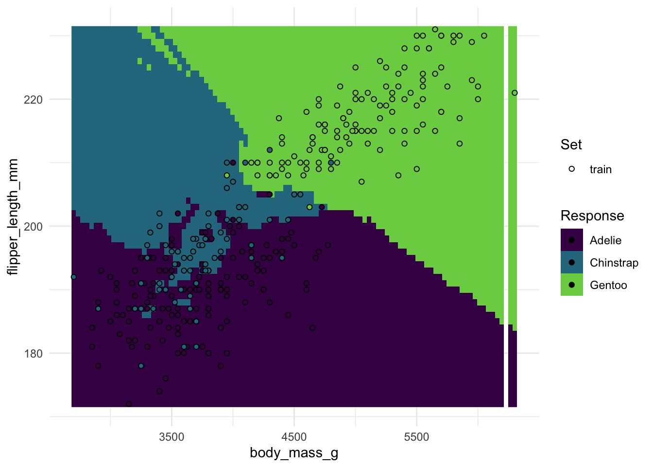
1.4 Your turn!
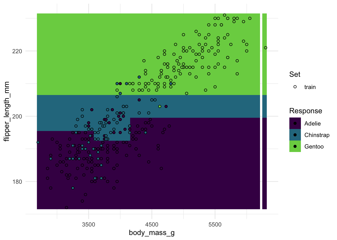
Now that we’ve done the kNN fitting with {mlr3}, you can easily do the same thing with the rpart-learner! All you have to do is switch the learner objects and give it a more fitting name.
# your code
Example solution
# Picking the learner
rpart_learner <- lrn("classif.rpart")

# What parameters does this learner have?
rpart_learner$param_set$ids()
#> [1] "cp" "keep_model" "maxcompete" "maxdepth"
#> [5] "maxsurrogate" "minbucket" "minsplit" "surrogatestyle"
#> [9] "usesurrogate" "xval"# Setting parameters (omit to use the defaults)
rpart_learner$param_set$values$maxdepth <- 20
# Train
rpart_learner$train(penguin_task, row_ids = penguin_split$train)
# Predict
rpart_prediction <- rpart_learner$predict(penguin_task, row_ids = penguin_split$test)
rpart_prediction$confusion#> truth
#> response Adelie Chinstrap Gentoo
#> Adelie 52 9 0
#> Chinstrap 5 3 0
#> Gentoo 2 3 37# Accuracy
rpart_prediction$score(msr("classif.acc"))#> classif.acc
#> 0.8288288plot_learner_prediction(rpart_learner, penguin_task)#> INFO [08:35:30.411] [mlr3] Applying learner 'classif.rpart' on task 'penguins' (iter 1/1)#> Warning: Raster pixels are placed at uneven horizontal intervals and will be shifted
#> ℹ Consider using `geom_tile()` instead.