library(ggplot2) # For plotting
library(kknn) # For kNN learner
library(rpart) # For decision tree learners
library(palmerpenguins) # For penguinskNN & Trees
Goals of this part:
- Taking a look at our example dataset
- Introduce kNN via
{kknn}and decision trees via{rpart} - Train some models, look at some results
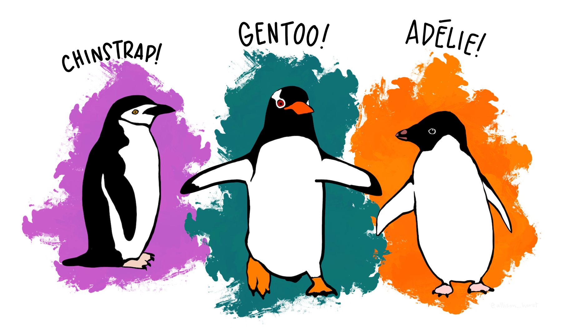
1 The dataset: Pengiuns!
See their website for some more information if you’re interested.
For now it’s enough to know that we have a bunch of data about 3 species of penguins.
# remove missing values for simplicity in this example
# (handling missing data is a can of worms for another time :)
penguins <- na.omit(penguins)

str(penguins)
#> tibble [333 × 8] (S3: tbl_df/tbl/data.frame)
#> $ species : Factor w/ 3 levels "Adelie","Chinstrap",..: 1 1 1 1 1 1 1 1 1 1 ...
#> $ island : Factor w/ 3 levels "Biscoe","Dream",..: 3 3 3 3 3 3 3 3 3 3 ...
#> $ bill_length_mm : num [1:333] 39.1 39.5 40.3 36.7 39.3 38.9 39.2 41.1 38.6 34.6 ...
#> $ bill_depth_mm : num [1:333] 18.7 17.4 18 19.3 20.6 17.8 19.6 17.6 21.2 21.1 ...
#> $ flipper_length_mm: int [1:333] 181 186 195 193 190 181 195 182 191 198 ...
#> $ body_mass_g : int [1:333] 3750 3800 3250 3450 3650 3625 4675 3200 3800 4400 ...
#> $ sex : Factor w/ 2 levels "female","male": 2 1 1 1 2 1 2 1 2 2 ...
#> $ year : int [1:333] 2007 2007 2007 2007 2007 2007 2007 2007 2007 2007 ...
#> - attr(*, "na.action")= 'omit' Named int [1:11] 4 9 10 11 12 48 179 219 257 269 ...
#> ..- attr(*, "names")= chr [1:11] "4" "9" "10" "11" ...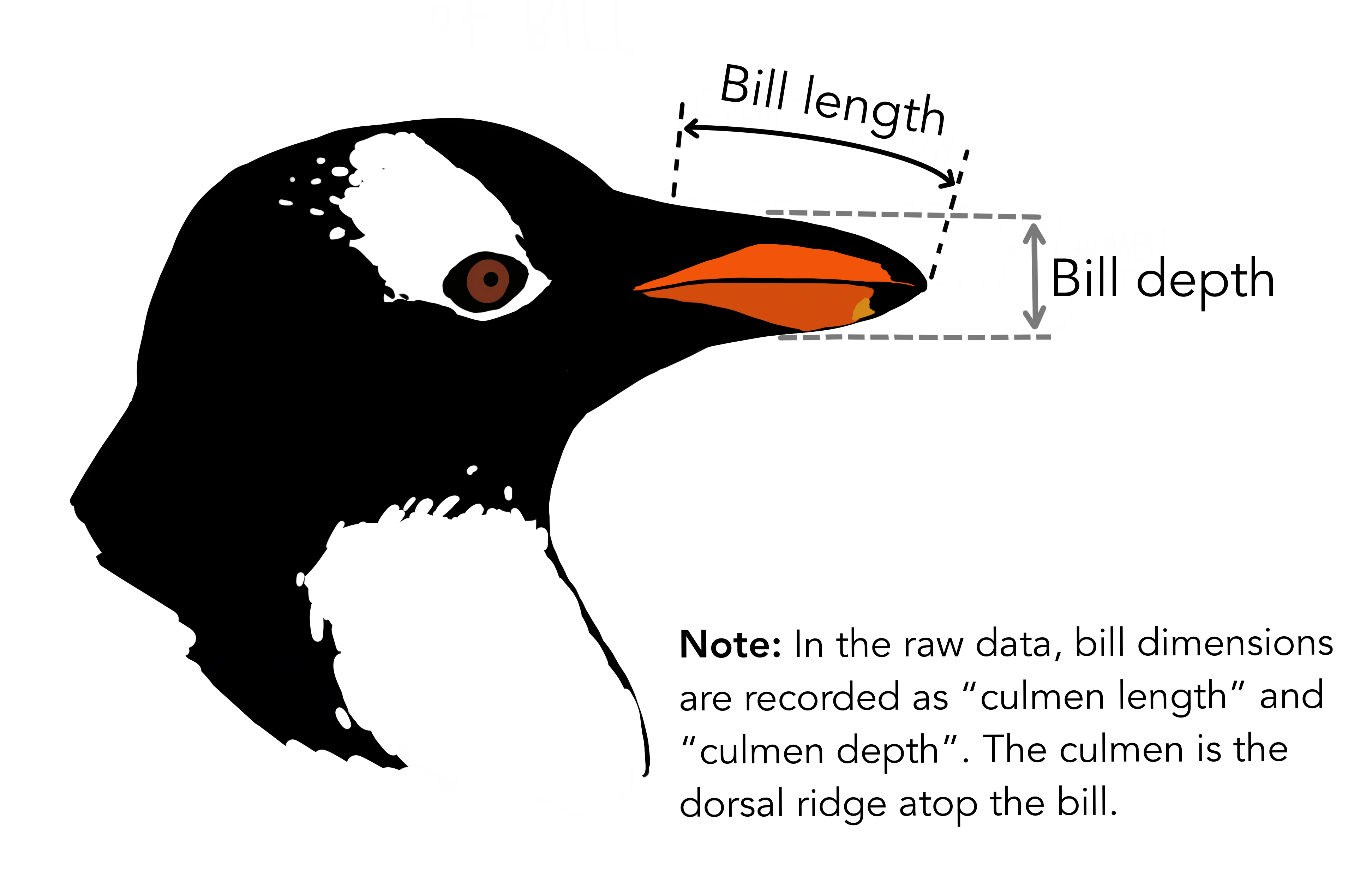
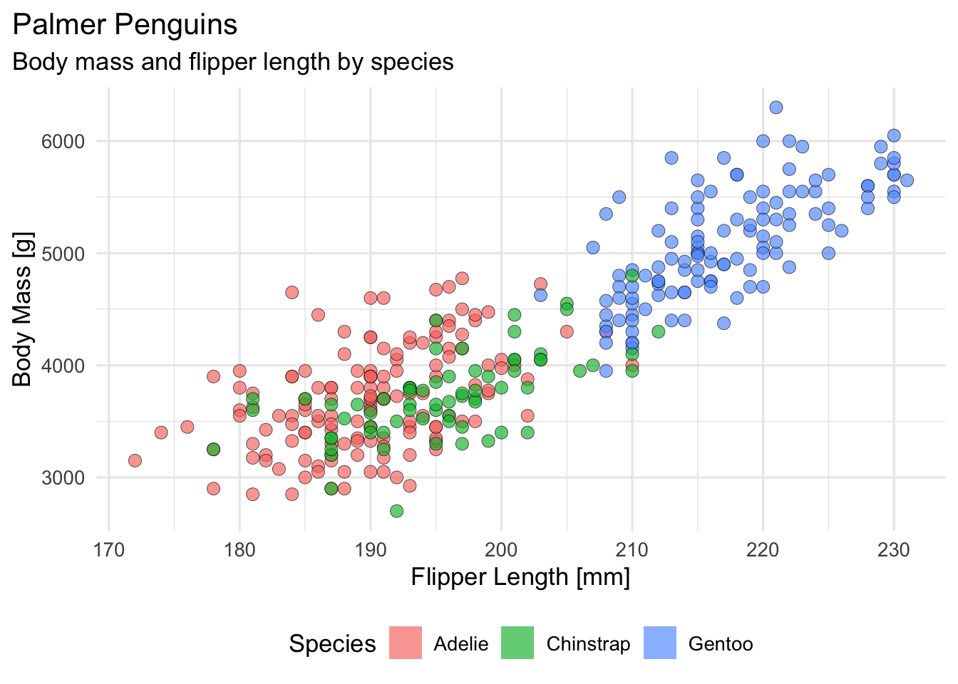
We can take a look at the different species across two numeric features, starting with flipper length and body mass (for reasons that may become clear later):
ggplot(penguins, aes(x = flipper_length_mm, y = body_mass_g, fill = species)) +
  # ggforce::geom_mark_ellipse(aes(fill = species, label = species)) +
  geom_point(
    shape = 21,
    stroke = 1 / 4,
    size = 3,
    alpha = 2 / 3,
    key_glyph = "rect"
  ) +
  labs(
    title = "Palmer Penguins",
    subtitle = "Body mass and flipper length by species",
    x = "Flipper Length [mm]",
    y = "Body Mass [g]",
    color = "Species",
    fill = "Species"
  ) +
  theme_minimal(base_size = 13) +
  theme(
    legend.position = "bottom",
    plot.title.position = "plot"
  )
Note
There are two penguins datasets:
penguinsfrom thepalmerpenguinsR package, which has been around for a whilepenguins, as included in R’sdatasetspackage as of recently, with slightly different variable names!
For backwards compatbility, we just assume the palmerpenguins version.
In the future, we will probably convert these materials
We split our penguin data in a roughly 2/3 to 1/3 training- and test dataset for our first experiments:
penguin_N <- nrow(penguins) # Our total sample size

# We draw 2/3 of all indices randomly with a sampling proportion of 2/3 with a fixed seed
set.seed(234)
train_ids <- sample(penguin_N, replace = FALSE, size = penguin_N * 2 / 3)
# Our test set are the indices not in the training set
test_ids <- setdiff(1:penguin_N, train_ids)

# Assemble our train/test set using the indices we just randomized
penguins_train <- penguins[train_ids, ]
penguins_test <- penguins[test_ids, ]
2 kNN and trees, step by step
Now that we have some data, we can start fitting models, just to see how it goes! Given the plot from earlier, we may have a rough idea that the flipper length and body mass measurements are already giving us a somewhat decent picture about the species.
2.1 kNN
Let’s start with the nearest-neighbor approach via the {kknn} package. It takes a formula argument like you may know from lm() and other common modeling functions in R, where the format is predict_this ~ on_this + and_that + ....
knn_penguins <- kknn(
  formula = species ~ flipper_length_mm + body_mass_g,
  k = 3, # Hyperparameter: How many neighbors to consider
  train = penguins_train, # Training data used to make predictions
  test = penguins_test # Data to make predictions on
)

# Peek at the predictions, one row per observation in test data
head(knn_penguins$prob)
#> Adelie Chinstrap Gentoo
#> [1,] 1.0000000 0.0000000 0
#> [2,] 0.3333333 0.6666667 0
#> [3,] 1.0000000 0.0000000 0
#> [4,] 0.3333333 0.6666667 0
#> [5,] 1.0000000 0.0000000 0
#> [6,] 1.0000000 0.0000000 0To get an idea of how well our predictions fit, we add them to our original test data and compare observed (true) and predicted species:
# Add predictions to the test dataset
penguins_test$knn_predicted_species <- fitted(knn_penguins)

# Rows: True species, columns: predicted species
table(
  penguins_test$species,
  penguins_test$knn_predicted_species,
  dnn = c("Observed", "Predicted")
)
#> Predicted
#> Observed Adelie Chinstrap Gentoo
#> Adelie 38 8 1
#> Chinstrap 12 8 4
#> Gentoo 0 1 39Proportion of correct predictions (“accuracy”)…
mean(penguins_test$species == penguins_test$knn_predicted_species)#> [1] 0.7657658…and incorrect predictions (classification error):
mean(penguins_test$species != penguins_test$knn_predicted_species)#> [1] 0.2342342
R shortcut
Logical comparison gives logical vector of TRUE/FALSE, which can be used like 1 / 0 for mathematical operations, so we can sum up cases where observed == predicted (=> correct classifications) and divide by N for the proportion, i.e. calculate the proportion of correct predictions, the accuracy.
2.2 Your turn!
Above you have working code for an acceptable but not great kNN model. Can you make it even better? Can you change something to make it worse?
Some things to try:
- Try different predictors, maybe leave some out
- Which seem to work best?
- Try using all available predictors (
formula = species ~ .)- Would you recommend doing that? Does it work well?
- Try different
kvalues. Is higher == better? (You can stick to odd numbers)- After you’ve tried a couple
k’s, does it get cumbersome yet?
- After you’ve tried a couple
# your code
knn_penguins <- kknn(
  formula = species ~ .,
  k = 7, # Hyperparameter: How many neighbors to consider
  train = penguins_train, # Training data used to make predictions
  test = penguins_test # Data to make predictions on
)
penguins_test$knn_predicted_species <- fitted(knn_penguins)
mean(penguins_test$species == penguins_test$knn_predicted_species)
#> [1] 1
Example solution
Already perfect accuracy with multiple predictors, not so interesting
knn_penguins <- kknn(
  formula = species ~ flipper_length_mm + body_mass_g + bill_length_mm + bill_depth_mm,
  k = 5,
  train = penguins_train,
  test = penguins_test
)

penguins_test$knn_predicted_species <- fitted(knn_penguins)
mean(penguins_test$species == penguins_test$knn_predicted_species)
#> [1] 1The “try a bunch of k”-shortcut function (using less features to be moderately interesting):
knn_try_k <- function(k) {
  knn_penguins <- kknn::kknn(
    formula = species ~ flipper_length_mm + body_mass_g + bill_depth_mm,
    k = k,
    train = penguins_train,
    test = penguins_test
  )

  penguins_test$knn_predicted_species <- fitted(knn_penguins)
  acc <- mean(penguins_test$species == penguins_test$knn_predicted_species)

  data.frame(k = k, accuracy = acc)
}

# Call function ^ with k = 1 through 10, collect result as data.frame
k_result <- do.call(rbind, lapply(1:10, knn_try_k))

ggplot(k_result, aes(x = k, y = accuracy)) +
  geom_line() +
  geom_point() +
  scale_x_continuous(breaks = 1:10) +
  scale_y_continuous(labels = scales::percent) +
  labs(
    title = "kNN test accuracy on penguin dataset",
    x = "k", y = "Test accuracy"
  ) +
  theme_minimal() +
  theme(panel.grid.minor = element_blank())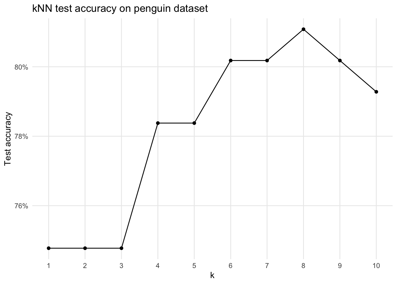
This is a cumbersome way to find the “best” k though — we’ll learn about the better ways later!
(We basically did a grid search across k here)
2.3 Growing a decision tree
Now that we’ve played around with kNN a little, let’s grow some trees! We’ll use the {rpart} (Recursive Partitioning) package and start with the same model specification as before and use the default parameters.
rpart_penguins <- rpart(
  formula = species ~ flipper_length_mm + body_mass_g,
  data = penguins_train, # Train data
  method = "class", # Grow a classification tree (don't change this for now)
)
The nice thing about a single tree is that you can just look at it and know exactly what it did:
rpart_penguins#> n= 222
#>
#> node), split, n, loss, yval, (yprob)
#> * denotes terminal node
#>
#> 1) root 222 123 Adelie (0.445945946 0.198198198 0.355855856)
#> 2) flipper_length_mm< 206.5 141 43 Adelie (0.695035461 0.297872340 0.007092199)
#> 4) flipper_length_mm< 194.5 96 19 Adelie (0.802083333 0.197916667 0.000000000) *
#> 5) flipper_length_mm>=194.5 45 22 Chinstrap (0.466666667 0.511111111 0.022222222)
#> 10) body_mass_g>=3762.5 29 12 Adelie (0.586206897 0.379310345 0.034482759)
#> 20) flipper_length_mm< 200.5 16 3 Adelie (0.812500000 0.187500000 0.000000000) *
#> 21) flipper_length_mm>=200.5 13 5 Chinstrap (0.307692308 0.615384615 0.076923077) *
#> 11) body_mass_g< 3762.5 16 4 Chinstrap (0.250000000 0.750000000 0.000000000) *
#> 3) flipper_length_mm>=206.5 81 3 Gentoo (0.012345679 0.024691358 0.962962963) *Looking at the tree as a… tree.
plot(rpart_penguins)
text(rpart_penguins)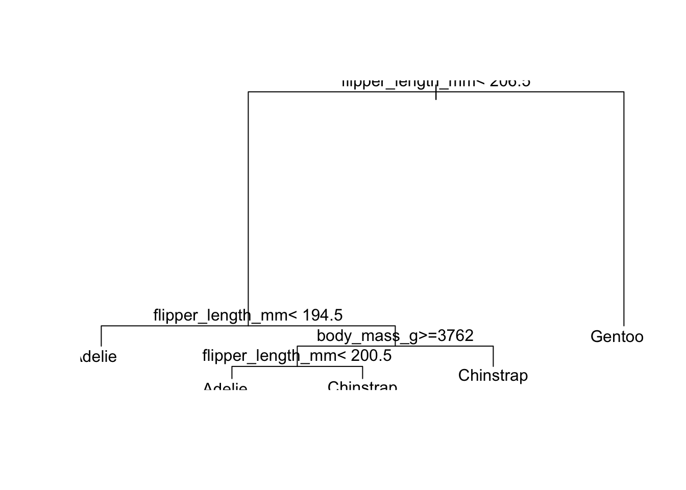
Much nicer to use the rpart.plot package though
library(rpart.plot)
rpart.plot(rpart_penguins)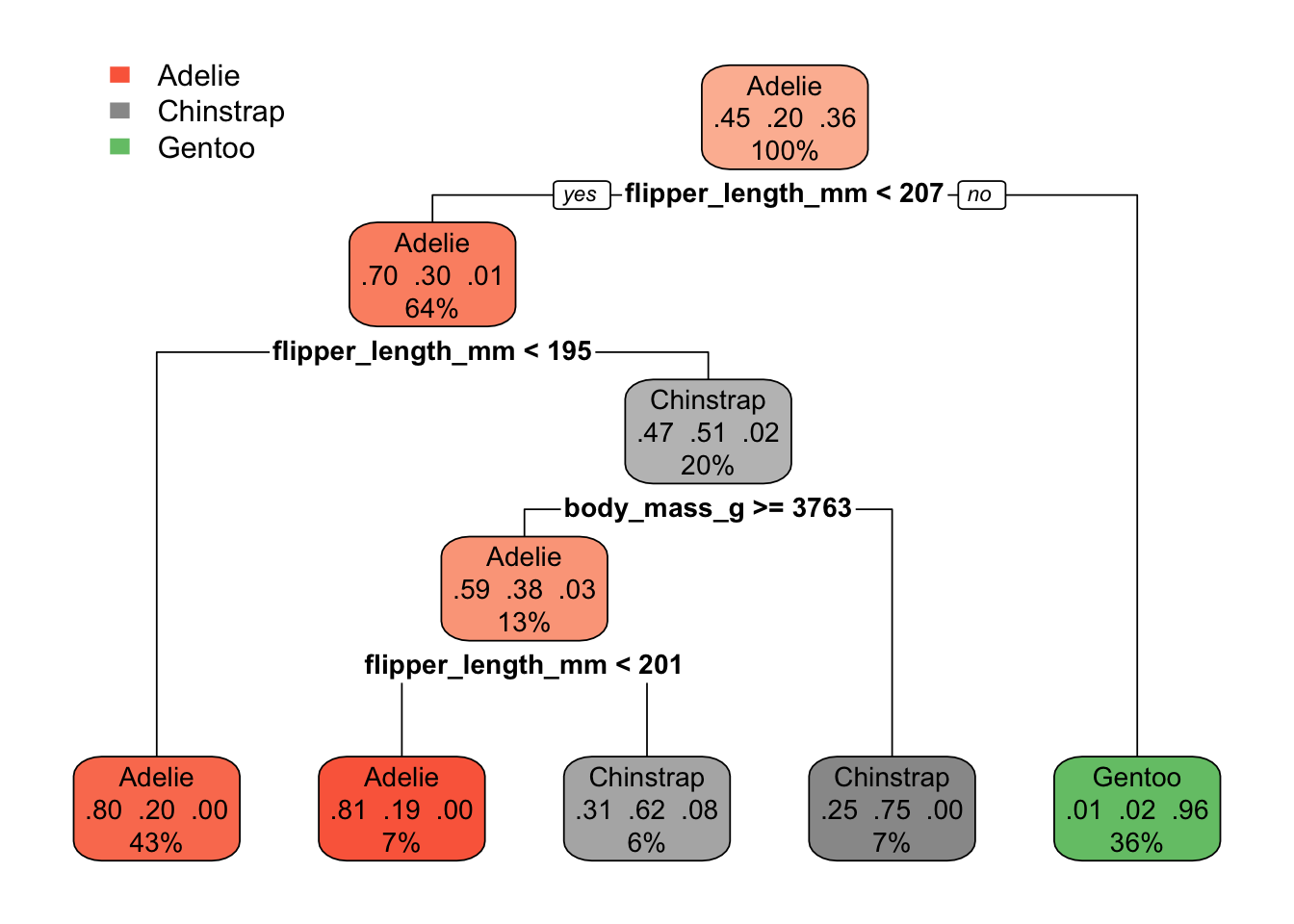
If we want to know how accurate we are with our model we need to make predictions on our test data manually:
rpart_predictions <- predict(
  rpart_penguins, # The model we just fit
  newdata = penguins_test, # New data to predict species on
  type = "class" # We want class predictions (the species), not probabilities
)

penguins_test$rpart_predicted_species <- rpart_predictions

# Same procedure as with kNN before
table(penguins_test$species, penguins_test$rpart_predicted_species)
#>
#> Adelie Chinstrap Gentoo
#> Adelie 40 6 1
#> Chinstrap 14 7 3
#> Gentoo 0 0 40# And our accuracy score
mean(penguins_test$species == penguins_test$rpart_predicted_species)#> [1] 0.78378382.4 Your turn!
We haven’t picked any hyperparameter settings for our tree yet, maybe we should try?
- What hyperparameters does
rpart()offer? Do you recognize some from the lecture?- You can check via
?rpart.control - When in doubt check
minsplit,maxdepthandcp
- You can check via
- Try out trees with different parameters
- Would you prefer simple or complex trees?
- How far can you improve the tree’s accuracy?
So, what seems to work better here?
kNN or trees?
# your code
Example solution
A “full” call to rpart with (most) relevant hyperparameters
rpart_penguins <- rpart(
  formula = species ~ flipper_length_mm + body_mass_g,
  data = penguins_train, # Train data
  method = "class", # Grow a classification tree (don't change this)
  cp = 0.03, # Complexity parameter for regularization (default = 0.01)
  minsplit = 15, # Number of obs to keep in node to continue splitting, default = 20
  minbucket = 2, # Number of obs to keep in terminal/leaf nodes, default is minsplit/3
  maxdepth = 15 # Maximum tree depth, default (and upper limit for rpart!) = 30
)

# Evaluate
penguins_test$rpart_predicted_species <- rpart_predictions
# Confusion matrix
table(penguins_test$species, penguins_test$rpart_predicted_species)
#>
#> Adelie Chinstrap Gentoo
#> Adelie 40 6 1
#> Chinstrap 14 7 3
#> Gentoo 0 0 40# Accuracy
mean(penguins_test$species == penguins_test$rpart_predicted_species)#> [1] 0.7837838Not much else to show here, just play around with the parameters!
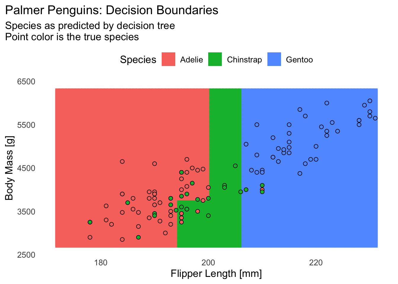
2.5 Plotting decision boundaries (for 2 predictors)
This is a rather cumbersome manual approach — there’s a nicer way we’ll see later, but we’ll do it the manual way at least once so you know how it works:
# Decision tree to plot the boundaries of
rpart_penguins <- rpart(
  formula = species ~ flipper_length_mm + body_mass_g,
  data = penguins_train, # Train data
  method = "class", # Grow a classification tree (don't change this)
  cp = 0.005, # Default 0.01
  minsplit = 20, # Default 20
  minbucket = 3, # Default is minsplit/3
  maxdepth = 30 # Default 30 (and upper limit!)
)

# Ranges of X and Y variable on plot
flipper_range <- range(penguins$flipper_length_mm)
mass_range <- range(penguins$body_mass_g)

# A grid of values within these boundaries, 100 points per axis
pred_grid <- expand.grid(
  flipper_length_mm = seq(flipper_range[1], flipper_range[2], length.out = 100),
  body_mass_g = seq(mass_range[1], mass_range[2], length.out = 100)
)

# Predict with tree for every single point
pred_grid$rpart_prediction <- predict(
  rpart_penguins,
  newdata = pred_grid,
  type = "class"
)

# Plot all predictions, colored by species
ggplot(pred_grid, aes(x = flipper_length_mm, y = body_mass_g)) +
  geom_tile(
    aes(color = rpart_prediction, fill = rpart_prediction),
    linewidth = 1,
    show.legend = FALSE
  ) +
  geom_point(
    data = penguins_test,
    aes(fill = species),
    shape = 21,
    color = "black",
    size = 2,
    key_glyph = "rect"
  ) +
  labs(
    title = "Palmer Penguins: Decision Boundaries",
    subtitle = paste(
      "Species as predicted by decision tree",
      "Point color is the true species",
      sep = "\n"
    ),
    x = "Flipper Length [mm]",
    y = "Body Mass [g]",
    fill = "Species"
  ) +
  theme_minimal(base_size = 13) +
  theme(
    legend.position = "top",
    plot.title.position = "plot",
    panel.grid = element_blank()
  )