library(mlr3verse) # Loads all the mlr3 stuff
library(ggplot2) # For plotting

# Just telling mlr3 to be quiet unless something broke
lgr::get_logger("mlr3")$set_threshold("error")Resampling, Random Forest & Boosting
Goals of this part:
- A Quick look at other tasks available and the “spam” task specifically
- Resampling for model evaluation
- Comparing learners with resampling
1 Task Setup
As we’ve seen last time, our penguin data is pretty easy for our learners. We need something a little more complex, meaning more observations (n) and a couple more predictors (p).
If you’re looking for ready-made example tasks for your own experimentation, mlr3 comes with a couple you can try. The procedure is similar to mlr_learners and mlr_measures, but this time it’s, you guessed it,
mlr_tasks#> <DictionaryTask> with 22 stored values
#> Keys: ames_housing, bike_sharing, boston_housing, breast_cancer,
#> california_housing, german_credit, ilpd, iris, kc_housing, moneyball,
#> mtcars, optdigits, penguins, penguins_simple, pima, ruspini, sonar,
#> spam, titanic, usarrests, wine, zoo# As a neat little table with all the relevant info
as.data.table(mlr_tasks)#> Key: <key>
#> key label task_type
#> <char> <char> <char>
#> 1: ames_housing Ames House Sales regr
#> 2: bike_sharing Bike Sharing Demand regr
#> 3: boston_housing Boston Housing Prices regr
#> 4: breast_cancer Wisconsin Breast Cancer classif
#> 5: california_housing California House Value regr
#> 6: german_credit German Credit classif
#> 7: ilpd Indian Liver Patient Data classif
#> 8: iris Iris Flowers classif
#> 9: kc_housing King County House Sales regr
#> 10: moneyball Major League Baseball Statistics regr
#> 11: mtcars Motor Trends regr
#> 12: optdigits Optical Recognition of Handwritten Digits classif
#> 13: penguins Palmer Penguins classif
#> 14: penguins_simple Simplified Palmer Penguins classif
#> 15: pima Pima Indian Diabetes classif
#> 16: ruspini Ruspini clust
#> 17: sonar Sonar: Mines vs. Rocks classif
#> 18: spam HP Spam Detection classif
#> 19: titanic Titanic classif
#> 20: usarrests US Arrests clust
#> 21: wine Wine Regions classif
#> 22: zoo Zoo Animals classif
#> key label task_type
#> nrow ncol properties lgl int dbl chr fct ord pxc dte
#> <int> <int> <list> <int> <int> <int> <int> <int> <int> <int> <int>
#> 1: 2930 82 0 33 1 0 47 0 0 0
#> 2: 17379 14 2 4 4 1 2 0 0 0
#> 3: 506 18 0 3 12 0 2 0 0 0
#> 4: 683 10 twoclass 0 0 0 0 0 9 0 0
#> 5: 20640 10 0 0 8 0 1 0 0 0
#> 6: 1000 21 twoclass 0 3 0 0 14 3 0 0
#> 7: 583 11 twoclass 0 4 5 0 1 0 0 0
#> 8: 150 5 multiclass 0 0 4 0 0 0 0 0
#> 9: 21613 20 1 13 4 0 0 0 1 0
#> 10: 1232 15 0 3 5 0 6 0 0 0
#> 11: 32 11 0 0 10 0 0 0 0 0
#> 12: 5620 65 twoclass 0 64 0 0 0 0 0 0
#> 13: 344 8 multiclass 0 3 2 0 2 0 0 0
#> 14: 333 11 multiclass 0 3 7 0 0 0 0 0
#> 15: 768 9 twoclass 0 0 8 0 0 0 0 0
#> 16: 75 2 0 2 0 0 0 0 0 0
#> 17: 208 61 twoclass 0 0 60 0 0 0 0 0
#> 18: 4601 58 twoclass 0 0 57 0 0 0 0 0
#> 19: 1309 11 twoclass 0 2 2 3 2 1 0 0
#> 20: 50 4 0 2 2 0 0 0 0 0
#> 21: 178 14 multiclass 0 2 11 0 0 0 0 0
#> 22: 101 17 multiclass 15 1 0 0 0 0 0 0
#> nrow ncol properties lgl int dbl chr fct ord pxc dteI suggest we try a two-class (i.e. binary) classification problem next, and maybe something we can probably all somewhat relate to: Spam detection.
spam_task <- tsk("spam")

# Outcome categories
spam_task$class_names
#> [1] "spam" "nonspam"# Target classes are not horribly unbalanced (40/60%)
autoplot(spam_task)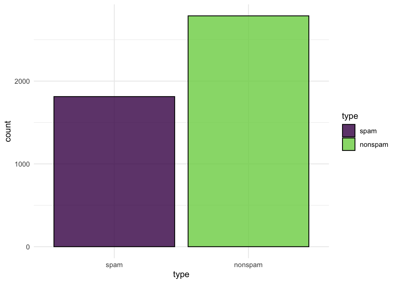
1.1 Your turn!
Explore the task a little (you can use its built-in methods spam_task$...) to check the data, get column types, the dataset dimensions etc. Think about this as a new analysis problem, so what do we need to know here?
(If you’d like a simpler overview, you can read the help with spam_task$help())
2 Resampling
To continue with our kNN and tree experiments, we’ll now enter resampling territory.
You probably realized that predicting on just one test dataset doesn’t give us too much of a useful idea of our model, which is why we use resampling.
There are lots of resampling strategies, but you usually can’t go too wrong with cross validation (CV), which should not take too much time and computing power on small datasets like ours.
Instead of training our model just once, we’re going to train it 5 times with different training- and test-datasets. In {mlr3}, we first pick a resampling strategy with rsmp(), and then define our setup with resample() based on our task and resampling strategy. The result an object of class ResampleResult:
rr <- resample(
  task = spam_task,
  # Optional: Adjust learner parameters
  learner = lrn("classif.kknn", k = 13, predict_sets = c("train", "test")),
  resampling = rsmp("cv", folds = 3) # 3-fold CV
)

rr
#>
#> ── <ResampleResult> with 3 resampling iterations ───────────────────────────────
#> task_id learner_id resampling_id iteration prediction_train
#> spam classif.kknn cv 1 <PredictionClassif>
#> spam classif.kknn cv 2 <PredictionClassif>
#> spam classif.kknn cv 3 <PredictionClassif>
#> prediction_test warnings errors
#> <PredictionClassif> 0 0
#> <PredictionClassif> 0 0
#> <PredictionClassif> 0 0# Contains task/learner/resampling/prediction objects
as.data.table(rr)#> task learner resampling
#> <list> <list> <list>
#> 1: <TaskClassif:spam> <LearnerClassifKKNN:classif.kknn> <ResamplingCV>
#> 2: <TaskClassif:spam> <LearnerClassifKKNN:classif.kknn> <ResamplingCV>
#> 3: <TaskClassif:spam> <LearnerClassifKKNN:classif.kknn> <ResamplingCV>
#> iteration prediction
#> <int> <list>
#> 1: 1 <PredictionClassif>
#> 2: 2 <PredictionClassif>
#> 3: 3 <PredictionClassif>We also tell our learner to predict both on train- and test sets.
Now we have a look at our predictions, but per resampling iteration, for both train- and test-set accuracy:
traintest_acc <- list(
  msr("classif.acc", predict_sets = "train", id = "acc_train"),
  msr("classif.acc", id = "acc_test")
)
rr$score(traintest_acc)[, .(iteration, acc_train, acc_test)]
#> iteration acc_train acc_test
#> <int> <num> <num>
#> 1: 1 0.9530486 0.9106910
#> 2: 2 0.9517444 0.9165580
#> 3: 3 0.9478488 0.9015003And on average over the resampling iterations:
rr$aggregate(traintest_acc)#> acc_train acc_test
#> 0.9508806 0.9095831As expected, our learner performed better on the training data than on the test data. By default, {mlr3} only gives us the results for the test data, which we’ll be focusing on going forward. Being able to compare train-/test-performance is useful though to make sure you’re not hopelessly overfitting on your training data!
Also note how we got to train our learner, do cross validation and get scores all without having to do any extra work. That’s why we use {mlr3} instead of doing everything manually — abstraction is nice.
Also note that we don’t always have to choose a measure, there’s a default measure for classification for example.
rr$aggregate()#> classif.ce
#> 0.090416882.1 One more thing: Measures
So far we’ve always used the accuracy, i.e. the proportion of correct classifications as our measure. For a problem such as spam detection that might not be the best choice, because it might be better to consider the probability that an e-mail is spam and maybe adjust the threshold at which we start rejecting mail.
For a class prediction we might say that if prob(is_spam) > 0.5 the message is classified as spam, but maybe we’d rather be more conservative and only consider a message to be spam at a probability over, let’s say, 70%. This will change the relative amounts of true and false positives and negatives:
knn_learner <- lrn("classif.kknn", predict_type = "prob", k = 13)

set.seed(123)
spam_split <- partition(spam_task)
knn_learner$train(spam_task, spam_split$train)
knn_pred <- knn_learner$predict(spam_task, spam_split$test)

# Measures: True Positive Rate (Sensitivity) and True Negative Rate (1 - Specificity)
measures <- msrs(c("classif.tpr", "classif.tnr"))
knn_pred$confusion
#> truth
#> response spam nonspam
#> spam 508 43
#> nonspam 95 872knn_pred$score(measures)#> classif.tpr classif.tnr
#> 0.8424544 0.9530055# Threshold of 70% probability of spam:
knn_pred$set_threshold(0.7)
knn_pred$confusion#> truth
#> response spam nonspam
#> spam 446 20
#> nonspam 157 895knn_pred$score(measures)#> classif.tpr classif.tnr
#> 0.7396352 0.9781421# If we were happy with only 20% probability of spam to mark a message as spam:
knn_pred$set_threshold(0.2)
knn_pred$confusion#> truth
#> response spam nonspam
#> spam 570 161
#> nonspam 33 754knn_pred$score(measures)#> classif.tpr classif.tnr
#> 0.9452736 0.8240437For a better analysis than just manually trying out different thresholds, we can use ROC curves.
To do so, we first have to adjust our Learner to predict the spam probability instead of already simplifying the prediction to "spam" or "nonspam". We use the autoplot() function based on the prediction, specifying type = "roc" to give us an ROC curve:
autoplot(knn_pred, type = "roc")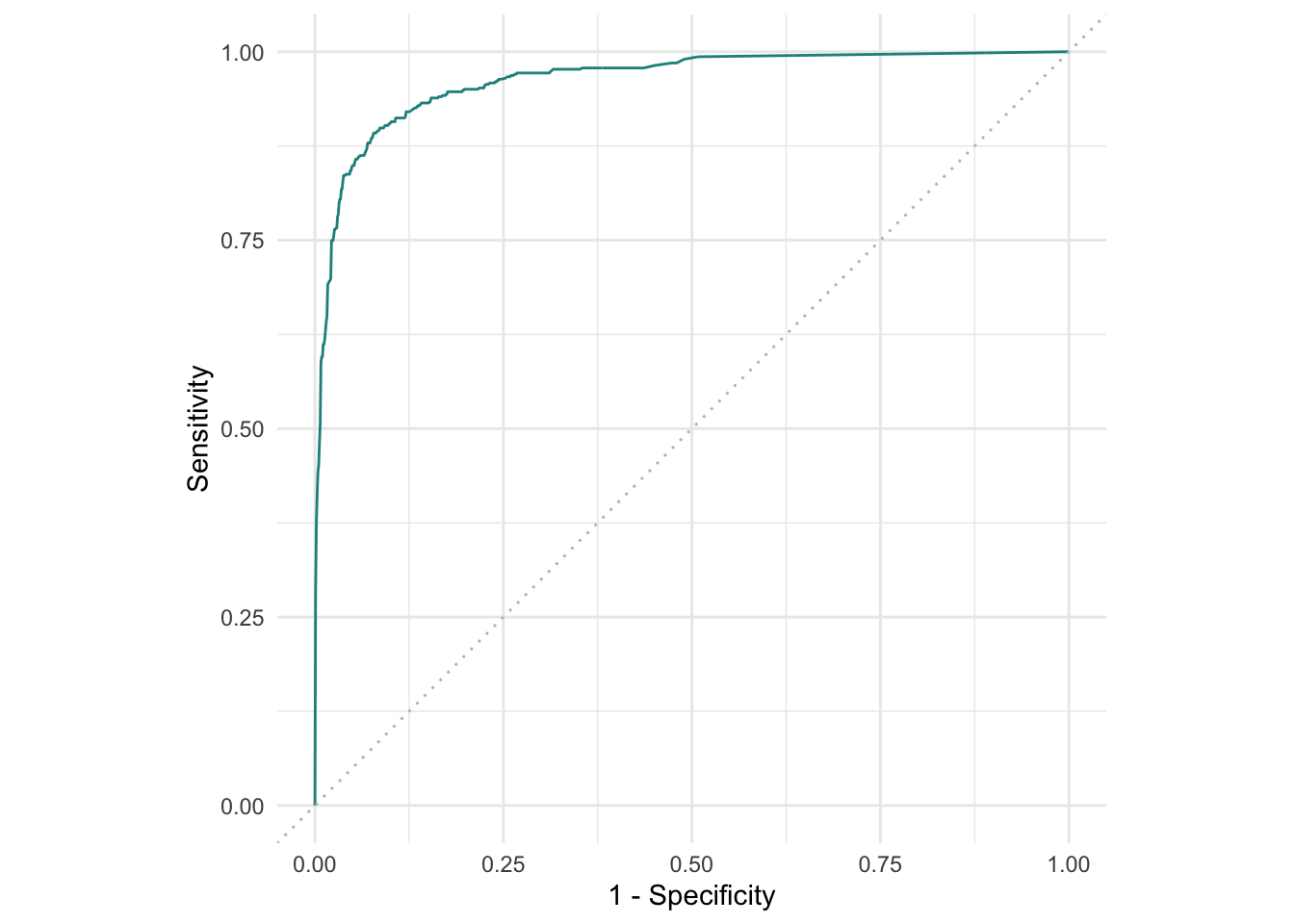
This gives us the false positive rate (FPR, “1 - Specificity”) and the Sensitivity (or true positive rate, TPR) for our binary classification example. “Positive” here means “the e-mail is spam”. If our classification model was basically a random coin flip, we would expect the curve to be the diagonal (depicted in grey in the plot). Everything in the upper-left is at least better than random.
To condense this to a single number, we use the AUC, the area under the (ROC) curve. If this AUC is 0.5, our model is basically a coin toss — and if it’s 1, that means our model is perfect, which is usually too good to be true and means we overfit in some way or the data is weird.
To get the AUC we use msr("classif.auc") instead of "classif.acc" going forward.
2.2 Your Turn!
- Repeat the same resampling steps for the
{rpart}decision tree learner. (Resample with 5-fold CV, evaluate based on test accuracy)
- Does it fare better than kNN with default parameters?
- Repeat either learner resampling with different hyperparameters
{mlr3viz}provides alternatives to the ROC curve, which are described in the help page?autoplot.PredictionClassif. Experiment with precision recall and threshold curves. Which would you consider most useful?
This is technically peck-and-find hyperparameter tuning which we’ll do in a more convenient (and methodologically sound) way in the next part :)
# your code
Example solution
The idea would be to re-run this code chunk with different hyperparameters:
rr <- resample(
  task = spam_task,
  # Important: set predict_type to "prob", set other parameters as desired.
  learner = lrn(
    "classif.rpart",
    predict_type = "prob",
    maxdepth = 15,
    cp = 0.003
  ),
  resampling = rsmp("cv", folds = 3)
)

rr$score(msr("classif.acc"))[, .(classif.acc)]
#> classif.acc
#> <num>
#> 1: 0.9022164
#> 2: 0.9211213
#> 3: 0.9197652ROC curve based on resampling iterations:
autoplot(rr, type = "roc")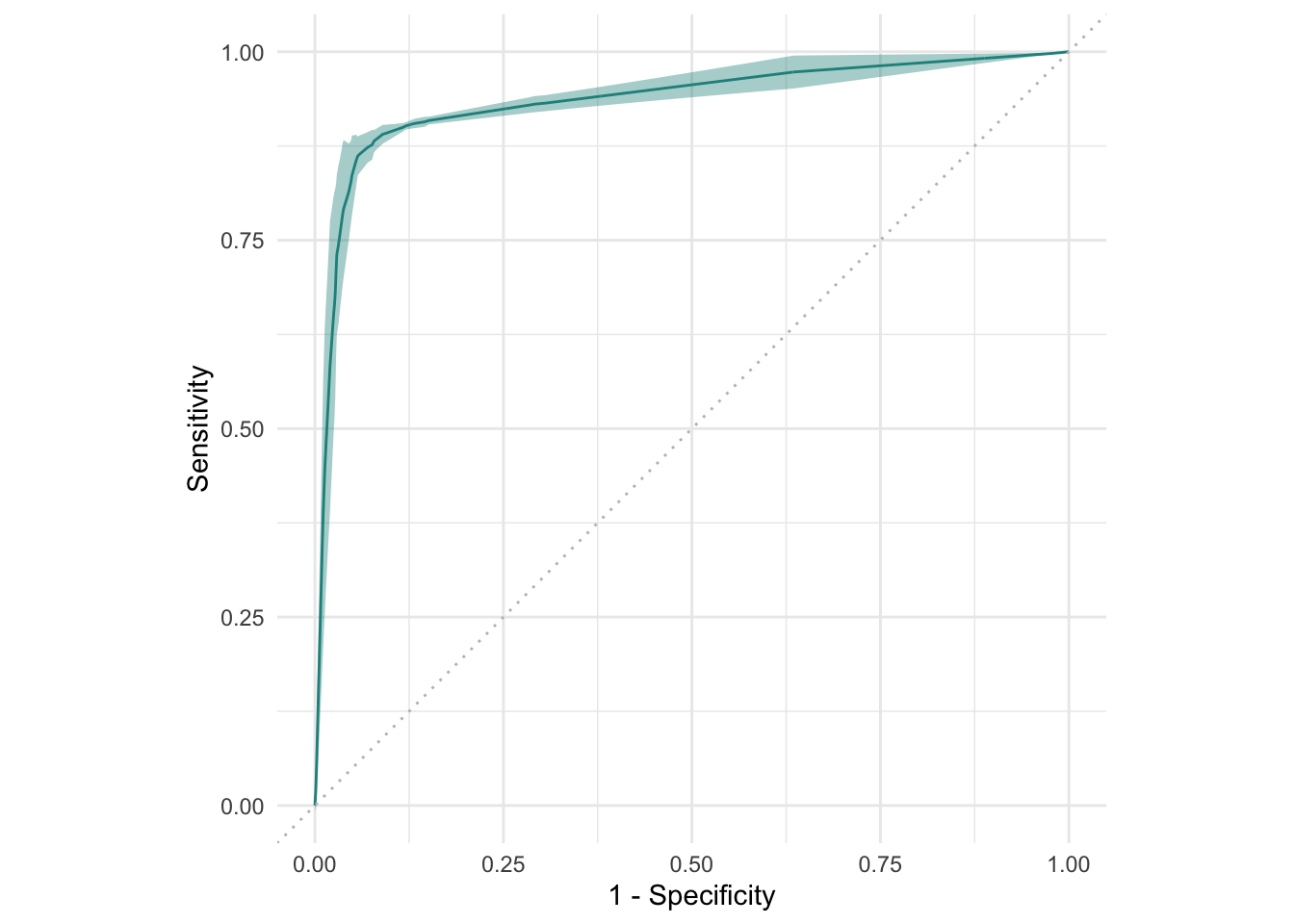
rr$aggregate(msr("classif.auc"))#> classif.auc
#> 0.934748Alternatives to ROC: Precision-Recall curve (prc) and a threshold-error curve — all three can be very useful depending on your specific classification problem!
autoplot(rr, type = "prc")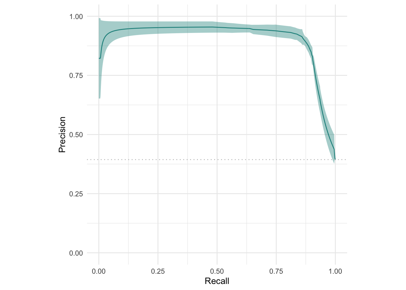
# Threshold plot doesn't work on resampling result, but on prediction objects!
autoplot(rr$prediction(), type = "threshold")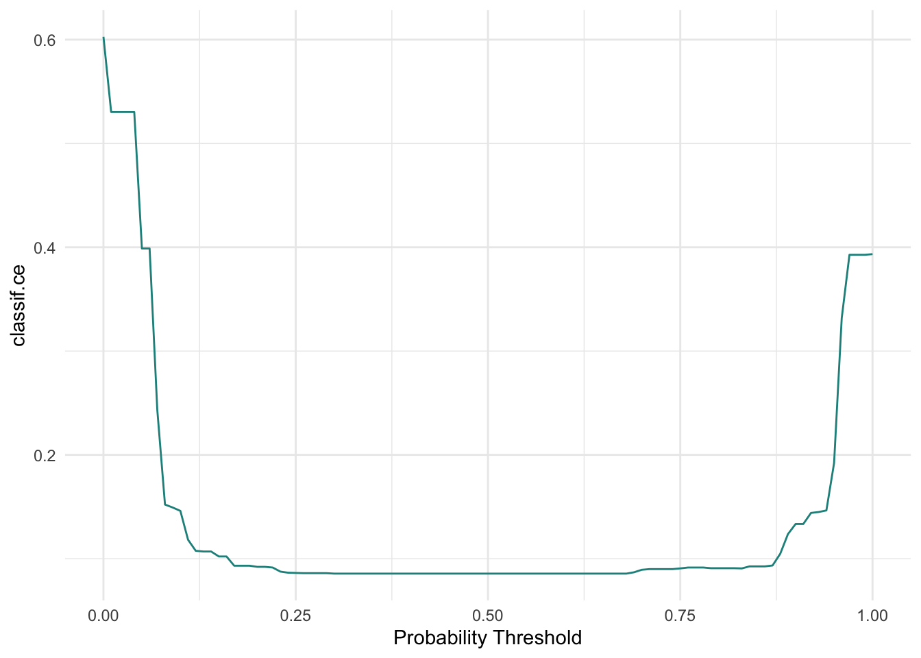
3 Benchmarking
The next thing we’ll try is to resample across multiple learners at once — because doing resampling for each learner separately and comparing results is just too tedious.
Let’s set up our learners with default parameters and compare them against a dummy featureless learner, which serves as a naive baseline. This learner always predicts the average of the target or the majority class in this case, so it’s the worst possible learner that should be beatable by any reasonable algorithm!
learners <- list(
  lrn("classif.kknn", id = "knn", predict_type = "prob"),
  lrn("classif.rpart", id = "tree", predict_type = "prob"),
  lrn("classif.featureless", id = "Baseline", predict_type = "prob")
)

# Define task, learners and resampling strategy in a benchmark design
design <- benchmark_grid(
  tasks = spam_task, # Still the same task
  learners = learners, # The new list of learners
  resamplings = rsmp("cv", folds = 3) # Same resampling strategy as before
)

# Run the benchmark and save the results ("BenchmarkResult" object)
bmr <- benchmark(design)
bmr
#>
#> ── <BenchmarkResult> of 9 rows with 3 resampling run ───────────────────────────
#> nr task_id learner_id resampling_id iters warnings errors
#> 1 spam knn cv 3 0 0
#> 2 spam tree cv 3 0 0
#> 3 spam Baseline cv 3 0 0# It's just a collection of ResampleResult objects from before!
as.data.table(bmr)#> uhash task
#> <char> <list>
#> 1: 618667dc-297e-47fd-9972-5d6eabb7e5eb <TaskClassif:spam>
#> 2: 618667dc-297e-47fd-9972-5d6eabb7e5eb <TaskClassif:spam>
#> 3: 618667dc-297e-47fd-9972-5d6eabb7e5eb <TaskClassif:spam>
#> 4: 93f718f0-107b-48c0-b6fd-8097d44569e8 <TaskClassif:spam>
#> 5: 93f718f0-107b-48c0-b6fd-8097d44569e8 <TaskClassif:spam>
#> 6: 93f718f0-107b-48c0-b6fd-8097d44569e8 <TaskClassif:spam>
#> 7: 74eb48a0-c4cc-443d-b58a-f17250b347e9 <TaskClassif:spam>
#> 8: 74eb48a0-c4cc-443d-b58a-f17250b347e9 <TaskClassif:spam>
#> 9: 74eb48a0-c4cc-443d-b58a-f17250b347e9 <TaskClassif:spam>
#> learner resampling iteration
#> <list> <list> <int>
#> 1: <LearnerClassifKKNN:knn> <ResamplingCV> 1
#> 2: <LearnerClassifKKNN:knn> <ResamplingCV> 2
#> 3: <LearnerClassifKKNN:knn> <ResamplingCV> 3
#> 4: <LearnerClassifRpart:tree> <ResamplingCV> 1
#> 5: <LearnerClassifRpart:tree> <ResamplingCV> 2
#> 6: <LearnerClassifRpart:tree> <ResamplingCV> 3
#> 7: <LearnerClassifFeatureless:Baseline> <ResamplingCV> 1
#> 8: <LearnerClassifFeatureless:Baseline> <ResamplingCV> 2
#> 9: <LearnerClassifFeatureless:Baseline> <ResamplingCV> 3
#> prediction task_id learner_id resampling_id
#> <list> <char> <char> <char>
#> 1: <PredictionClassif> spam knn cv
#> 2: <PredictionClassif> spam knn cv
#> 3: <PredictionClassif> spam knn cv
#> 4: <PredictionClassif> spam tree cv
#> 5: <PredictionClassif> spam tree cv
#> 6: <PredictionClassif> spam tree cv
#> 7: <PredictionClassif> spam Baseline cv
#> 8: <PredictionClassif> spam Baseline cv
#> 9: <PredictionClassif> spam Baseline cvbmr contains everything we’d like to know about out comparison. We extract the scores and take a look:
bm_scores <- bmr$score(msr("classif.auc"))
bm_scores
#> nr task_id learner_id resampling_id iteration prediction_test
#> <int> <char> <char> <char> <int> <list>
#> 1: 1 spam knn cv 1 <PredictionClassif>
#> 2: 1 spam knn cv 2 <PredictionClassif>
#> 3: 1 spam knn cv 3 <PredictionClassif>
#> 4: 2 spam tree cv 1 <PredictionClassif>
#> 5: 2 spam tree cv 2 <PredictionClassif>
#> 6: 2 spam tree cv 3 <PredictionClassif>
#> 7: 3 spam Baseline cv 1 <PredictionClassif>
#> 8: 3 spam Baseline cv 2 <PredictionClassif>
#> 9: 3 spam Baseline cv 3 <PredictionClassif>
#> classif.auc
#> <num>
#> 1: 0.9670819
#> 2: 0.9522196
#> 3: 0.9553746
#> 4: 0.9150956
#> 5: 0.8761300
#> 6: 0.8906025
#> 7: 0.5000000
#> 8: 0.5000000
#> 9: 0.5000000
#> Hidden columns: uhash, task, learner, resampling# Extract per-iteration accuracy per learner (only first five rows shows)
bm_scores[1:5, .(learner_id, iteration, classif.auc)]#> learner_id iteration classif.auc
#> <char> <int> <num>
#> 1: knn 1 0.9670819
#> 2: knn 2 0.9522196
#> 3: knn 3 0.9553746
#> 4: tree 1 0.9150956
#> 5: tree 2 0.8761300# To get all results for the tree learner
bm_scores[learner_id == "tree", .(learner_id, iteration, classif.auc)]#> learner_id iteration classif.auc
#> <char> <int> <num>
#> 1: tree 1 0.9150956
#> 2: tree 2 0.8761300
#> 3: tree 3 0.8906025# Or the results of the first iteration
bm_scores[iteration == 1, .(learner_id, iteration, classif.auc)]#> learner_id iteration classif.auc
#> <char> <int> <num>
#> 1: knn 1 0.9670819
#> 2: tree 1 0.9150956
#> 3: Baseline 1 0.5000000And if we want to see what worked best overall:
bmr$aggregate(msr("classif.auc"))[, .(learner_id, classif.auc)]#> learner_id classif.auc
#> <char> <num>
#> 1: knn 0.9582254
#> 2: tree 0.8939427
#> 3: Baseline 0.5000000autoplot(bmr, measure = msr("classif.auc"))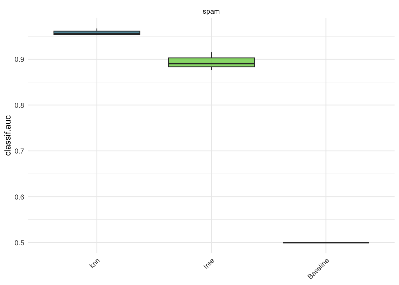
autoplot(bmr, type = "roc")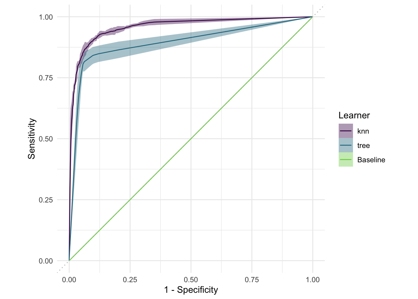
We see what we’d expect regarding the featureless learner — it’s effectively a coin toss. Also, kNN does quite a bit better than the decision tree with the default parameters here.
Of course including the featureless learner here doesn’t really add any insights, especially since we evaluate by AUC, where the featureless learner gets a score of 0.5 by definition.
3.1 Your Turn!
Since we have a binary classification problem, we might even get away with using plain old logistic regression.
Instead of benchmarking against the featureless learner, compare kNN and decision trees to the logistic regression learner "classif.log_reg" without any hyperparameters.
Do our fancy ML methods beat the good old GLM? Use the best hyperparameter settings for kNN and rpart you have found so far
# your code
Example solution
learners <- list(
  lrn("classif.kknn", id = "knn", predict_type = "prob", k = 25),
  lrn("classif.rpart", id = "tree", predict_type = "prob", maxdepth = 11, cp = 0.0036),
  lrn("classif.log_reg", id = "LogReg", predict_type = "prob")
)

design <- benchmark_grid(
  tasks = spam_task,       # Still the same task
  learners = learners,     # The new list of learners
  resamplings = rsmp("cv", folds = 3)  # Same resampling strategy as before
)

# Run the benchmark and save the results
bmr <- benchmark(design)
#> Warning: glm.fit: fitted probabilities numerically 0 or 1 occurred
#> Warning: glm.fit: fitted probabilities numerically 0 or 1 occurred
#> Warning: glm.fit: fitted probabilities numerically 0 or 1 occurredautoplot(bmr, type = "roc")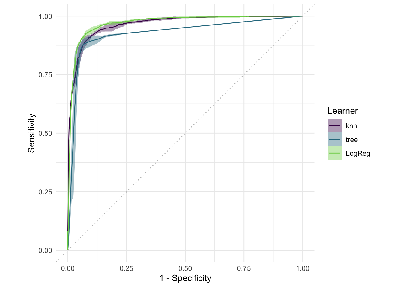
bmr$aggregate(msr("classif.auc"))[, .(learner_id, classif.auc)]#> learner_id classif.auc
#> <char> <num>
#> 1: knn 0.9654111
#> 2: tree 0.9276236
#> 3: LogReg 0.97078104 Random Forests & Boosting
Armed with our new model comparison skills, we can add Random Forests and Gradient Boosting to the mix!
Our new learner IDs are
"classif.ranger"for Random Forest, see?ranger::ranger"classif.xgboost"for (eXtreme) Gradient Boosting, see?xgboost::xgboost
(You know it has to be fancy if it has “extreme” in the name!)
Both learners can already do fairly well without tweaking hyperparameters, except for the nrounds value in xgboost which sets the number of boosting iterations. The default in the {mlr3} learner is 1, which kind of defeats the purpose of boosting.
4.1 Your Turn!
Use the benchmark setup from above and switch the kknn and rpart learners with the Random Forest and Boosting learners.
Maybe switch to holdout resampling to speed the process up a little and make sure to set nrounds to something greater than 1 for xgboost.
What about now? Can we beat logistic regression?
# your code
Example solution
learners <- list(
  lrn("classif.ranger", id = "forest", predict_type = "prob"),
  lrn("classif.xgboost", id = "xgboost", predict_type = "prob", nrounds = 5),
  lrn("classif.log_reg", id = "LogReg", predict_type = "prob")
)

design <- benchmark_grid(
  tasks = spam_task,       # Still the same task
  learners = learners,     # The new list of learners
  resamplings = rsmp("cv", folds = 3)
)

# Run the benchmark and save the results
bmr <- benchmark(design)
#> Warning: glm.fit: fitted probabilities numerically 0 or 1 occurred
#> Warning: glm.fit: fitted probabilities numerically 0 or 1 occurred
#> Warning: glm.fit: fitted probabilities numerically 0 or 1 occurredautoplot(bmr, type = "roc")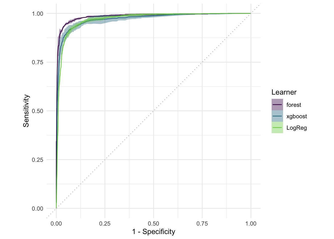
bmr$aggregate(msr("classif.auc"))[, .(learner_id, classif.auc)]#> learner_id classif.auc
#> <char> <num>
#> 1: forest 0.9847315
#> 2: xgboost 0.9703650
#> 3: LogReg 0.9696380