Tuning

Last Updated

July 16, 2025

library(mlr3verse) # All the mlr3 things
library(ggplot2) # For plotting
lgr::get_logger("mlr3")$set_threshold("error")

# Spam Task setup
spam_task <- tsk("spam")
set.seed(26)

# train/test split
spam_split <- partition(spam_task, ratio = 2 / 3)

Goals of this part:

Introduce hyperparameter tuning
Experiment with tuning different learners

1 Hyperparameter Tuning

So far we’ve seen four learners:

kNN via {kknn}
Decision Trees via {rpart}
Random Forest via {ranger}
Gradient Boosting via {xgboost}

We’ve gotten to know the first two a little, and now we’ll also take a closer look at the second two.

First we’ll start doing some tuning with {mlr3} based on the kNN learner because it’s nice and simple. We saw that k is an important parameter, and it’s an integer greater than 1 at least. To tune it, we also have to make a few other decisions, also using what we learned about (nested) resampling.

What’s our resampling strategy?
What measure to we tune on?
What does the parameter search space look like?
How long to we tune? What’s our budget?
What’s our tuning strategy?

We’ll use {mlr3}’s auto_tuner for this because it’s just so convenient:

# Defining a search space: k is an integer, we look in range 3 to 51
search_space_knn = ps(
  k = p_int(lower = 3, upper = 51)
)

tuned_knn <- auto_tuner(
  # The base learner we want to tune, optionally setting other parameters
  learner = lrn("classif.kknn", predict_type = "prob"),
  # Resampling strategy for the tuning (inner resampling)
  resampling = rsmp("cv", folds = 3),
  # Tuning measure: Maximize the classification accuracy
  measure = msr("classif.bbrier"),
  # Setting the search space we defined above
  search_space = search_space_knn,
  # Budget: Try n_evals different values
  terminator = trm("evals", n_evals = 20),
  # Strategy: Randomly try parameter values in the space
  # (not ideal in this case but in general a good place to start)
  tuner = tnr("random_search")
)

# Take a look at the new tuning learner
tuned_knn

#> 
#> ── <AutoTuner> (classif.kknn.tuned) ────────────────────────────────────────────
#> • Model: -
#> • Parameters: list()
#> • Packages: mlr3, mlr3tuning, mlr3learners, and kknn
#> • Predict Types: response and [prob]
#> • Feature Types: logical, integer, numeric, factor, and ordered
#> • Encapsulation: none (fallback: -)
#> • Properties: multiclass and twoclass
#> • Other settings: use_weights = 'error'
#> • Search Space:
#>        id    class lower upper nlevels
#>    <char>   <char> <num> <num>   <num>
#> 1:      k ParamInt     3    51      49

Now tuned_knn behaves the same way as any other Learner that has not been trained on any data yet — first we have to train (and tune!) it on our spam training data. The result will be the best hyperparameter configuration of those we tried:

# If you're on your own machine with multiple cores available, you can parallelize:
future::plan("multisession", workers = 4)

# Setting a seed so we get the same results -- train on train set only!
set.seed(2398)
tuned_knn$train(spam_task, row_ids = spam_split$train)

(Side task: Try the same but with the AUC measure — do you get the same k?)

We can visualize the performance across all values of k we tried by accessing the tuning instance now included in the tuned_knn learner object:

autoplot(tuned_knn$tuning_instance)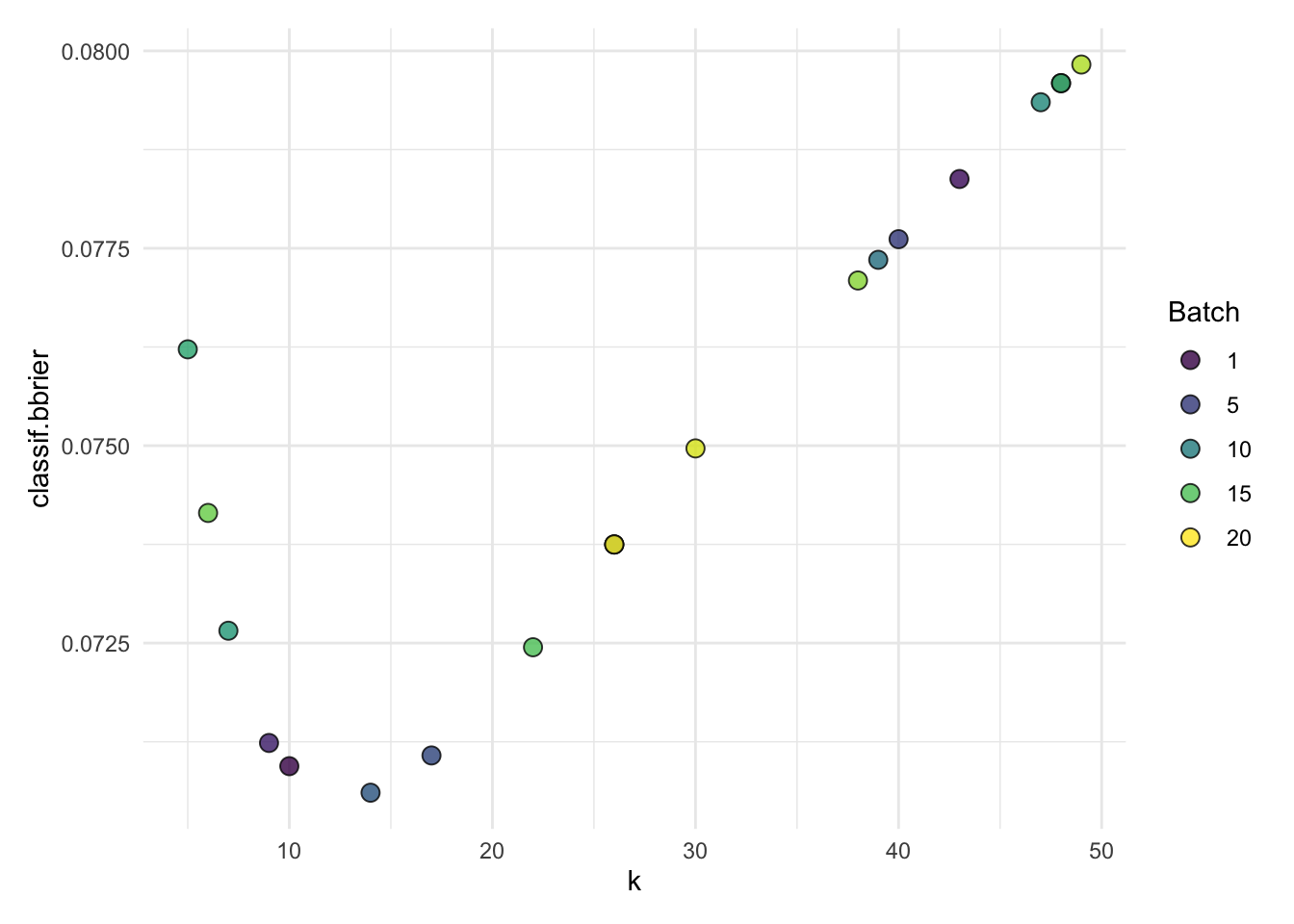

tuned_knn$tuning_instance

#> 
#> ── <TuningInstanceBatchSingleCrit> ─────────────────────────────────────────────
#> • State: Optimized
#> • Objective: <ObjectiveTuningBatch>
#> • Search Space:
#>        id    class lower upper nlevels
#>    <char>   <char> <num> <num>   <num>
#> 1:      k ParamInt     3    51      49
#> • Terminator: <TerminatorEvals> (n_evals=20, k=0)
#> • Result:
#>        k classif.bbrier
#>    <int>          <num>
#> 1:    14     0.07060497
#> • Archive:
#>     classif.bbrier     k
#>              <num> <int>
#>  1:           0.07    10
#>  2:           0.08    43
#>  3:           0.07     9
#>  4:           0.08    48
#>  5:           0.08    40
#>  6:           0.07    17
#>  7:           0.07    14
#>  8:           0.07    26
#>  9:           0.08    39
#> 10:           0.07    26
#> 11:           0.08    47
#> 12:           0.07     7
#> 13:           0.08     5
#> 14:           0.08    48
#> 15:           0.07    22
#> 16:           0.07     6
#> 17:           0.08    38
#> 18:           0.08    49
#> 19:           0.07    30
#> 20:           0.07    26
#>     classif.bbrier     k

(See also docs at ?mlr3viz:::autoplot.TuningInstanceSingleCrit)

And we can get the hyperparameter results that worked best in the end:

tuned_knn$tuning_result

#>        k learner_param_vals  x_domain classif.bbrier
#>    <int>             <list>    <list>          <num>
#> 1:    14          <list[1]> <list[1]>     0.07060497

Now that we’ve tuned on the training set, it’s time to evaluate on the test set:

tuned_knn_pred <- tuned_knn$predict(spam_task, row_ids = spam_split$test)

# Accuracy and AUC
tuned_knn_pred$score(msrs(c("classif.acc", "classif.auc", "classif.bbrier")))

#>    classif.acc    classif.auc classif.bbrier 
#>     0.90482399     0.96285949     0.07076836

That was basically the manual way of doing nested resampling with an inner resampling strategy (CV) and an outer resampling strategy of holdout (the spam_train and spam_test sets).

In the next step we’re going to compare the knn learner with the decision tree learner, and for that we need a proper nested resampling:

# Set up the knn autotuner again
tuned_knn <- auto_tuner(
  # The base learner we want to tune, optionally setting other parameters
  learner = lrn("classif.kknn", predict_type = "prob"),
  # Resampling strategy for the tuning (inner resampling)
  resampling = rsmp("cv", folds = 3),
  # Tuning measure: Maximize the classification accuracy
  measure = msr("classif.bbrier"),
  # Setting the search space we defined above
  search_space = ps(k = p_int(lower = 3, upper = 51)),
  # Budget: Try n_evals different values
  terminator = trm("evals", n_evals = 20),
  # Strategy: Randomly try parameter values in the space
  # (not ideal in this case but in general a good place to start)
  tuner = tnr("random_search")
)

# Set up resampling with the ready-to-be-tuned learner and outer resampling: CV
knn_nested_tune <- resample(
  task = spam_task,
  learner = tuned_knn,
  resampling = rsmp("cv", folds = 3), # this is effectively the outer resampling
  store_models = TRUE
)

# Extract inner tuning results, since we now tuned in multiple CV folds
# Folds might conclude different optimal k
# AUC is averaged over inner folds
extract_inner_tuning_results(knn_nested_tune)

#>    iteration     k classif.bbrier learner_param_vals  x_domain task_id
#>        <int> <int>          <num>             <list>    <list>  <char>
#> 1:         1    16     0.07293843          <list[1]> <list[1]>    spam
#> 2:         2    16     0.07697195          <list[1]> <list[1]>    spam
#> 3:         3    14     0.07406681          <list[1]> <list[1]>    spam
#>            learner_id resampling_id
#>                <char>        <char>
#> 1: classif.kknn.tuned            cv
#> 2: classif.kknn.tuned            cv
#> 3: classif.kknn.tuned            cv

# Above combined individual results also accessible via e.g.
knn_nested_tune$learners[[2]]$tuning_result

#>        k learner_param_vals  x_domain classif.bbrier
#>    <int>             <list>    <list>          <num>
#> 1:    16          <list[1]> <list[1]>     0.07697195

# Plot of inner folds
autoplot(knn_nested_tune$learners[[1]]$tuning_instance)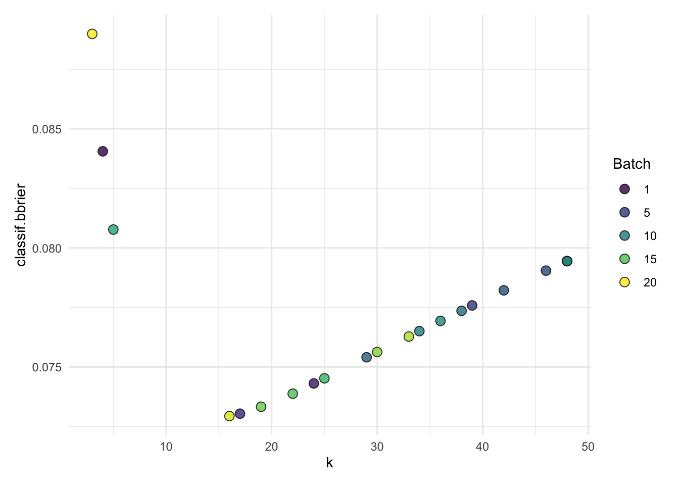

autoplot(knn_nested_tune$learners[[2]]$tuning_instance)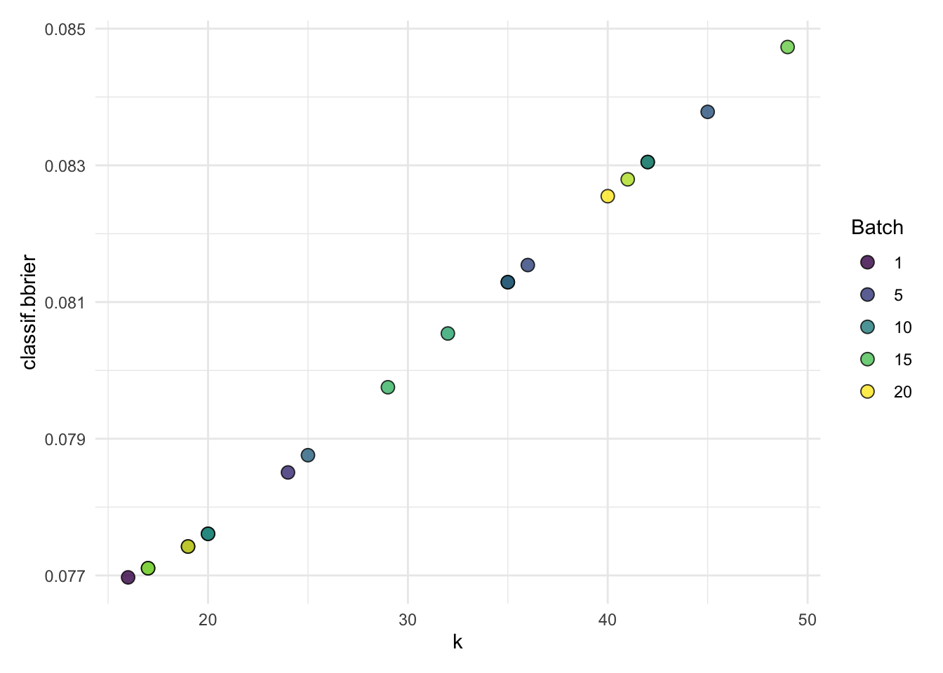

autoplot(knn_nested_tune$learners[[3]]$tuning_instance)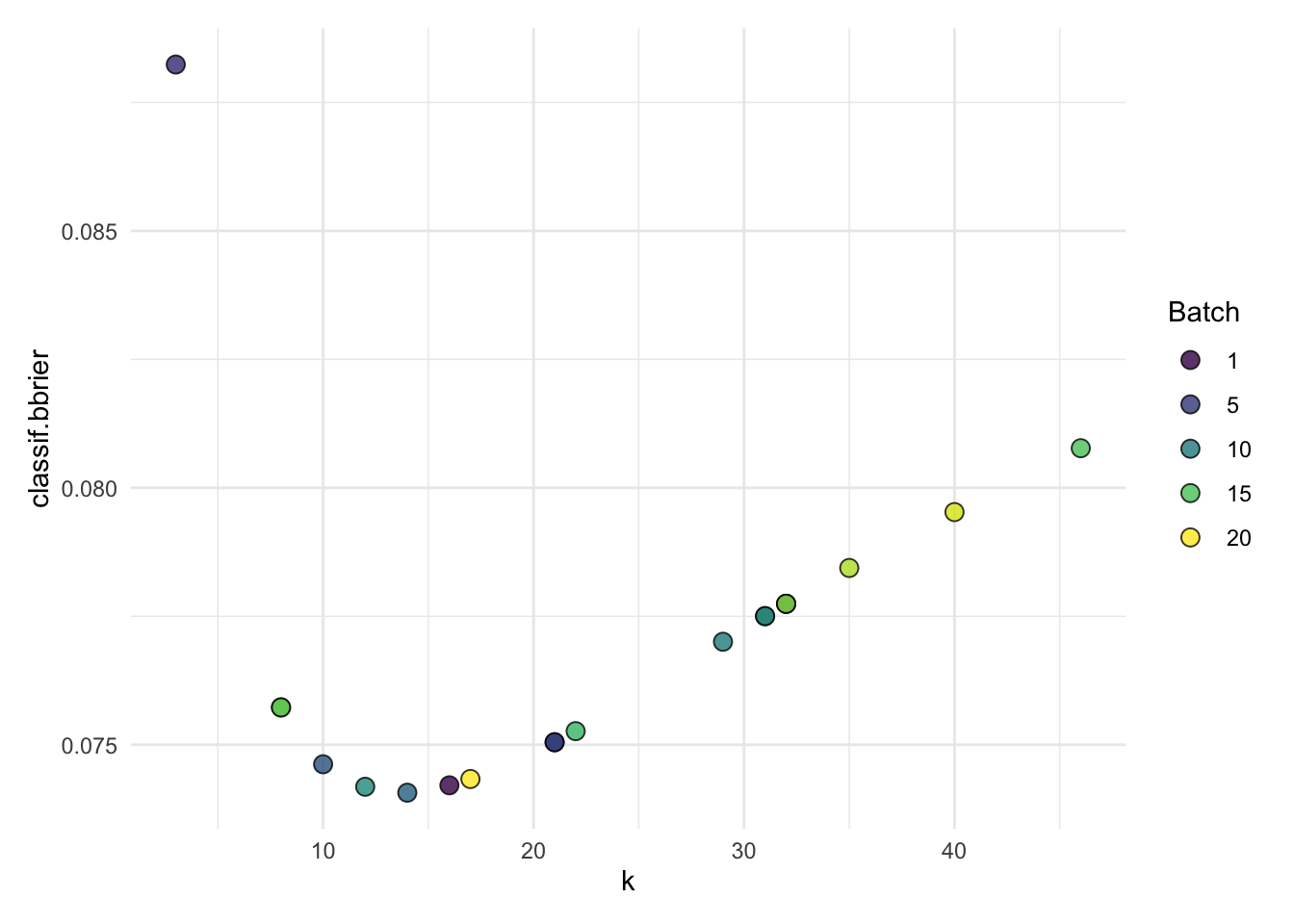

# Get AUC and acc for outer folds
knn_nested_tune$score(msrs(c("classif.acc", "classif.auc")))[, .(
  iteration,
  classif.auc,
  classif.acc
)]

#>    iteration classif.auc classif.acc
#>        <int>       <num>       <num>
#> 1:         1   0.9637586   0.9087353
#> 2:         2   0.9707207   0.9217731
#> 3:         3   0.9613927   0.9034573

# Average over outer folds - our "final result" performance for kNN
# AUC is averaged over outer folds
knn_nested_tune$aggregate(msrs(c("classif.acc", "classif.auc")))

#> classif.acc classif.auc 
#>   0.9113219   0.9652906

Seems like a decent result? Let’s try to beat it with some other learner!

1.1 Your Turn!

Above you have a boilerplate to tune your own learner. Start with either of the other three learners we’ve seen, pick one ore two hyperparameters to tune with a reasonable budget (note we have limited time and resources), tune on the training set and evaluate per AUC on the test set.

Some pointers:

Consult the Learner docs to see tuning-worthy parameters:
- lrn("classif.xgboost")$help() links to the xgboost help
- lrn("classif.rpart")$help() analogously for the decision tree
- You can also see the documentation online, e.g. https://mlr3learners.mlr-org.com/reference/mlr_learners_classif.xgboost.html
Parameter search spaces in ps() have different types, see the help at ?paradox::Domain
- Use p_int() for integers, p_dbl() for real-valued params etc.
If you don’t know which parameter to tune, try the following:
- classif.xgboost:
  - Important: nrounds (integer) (>= 1 (at least 50 or so))
  - Important: eta (double) (0 < eta < 1 (close to 0 probably))
  - Maybe: max_depth (integer)
- classif.rpart:
  - cp (double)
  - Maybe: maxdepth (integer) (< 30)
- classif.ranger:
  - mtry (integer) -> tune mtry.ratio (0 < mtry.ratio < 1)
  - max.depth (integer)

Note: Instead of randomly picking parameters from the design space, we can also generate a grid of parameters and try those. We’ll not try that here for now, but you can read up on how to do that here: ?mlr_tuners_grid_search.

-> generate_design_grid(search_space, resolution = 5)

Also note that the cool thing about the auto_tuner() is that it behaves just like any other mlr3 learner, but it automatically tunes itself. You can plug it into resample() or benchmark_grid() just fine!

# your code

Example solution

The following example code uses the holdout resampling just to keep it fast — when you have the time, using cross-validation ("cv") will give you more reliable results.

We also use 6 threads for parallelization here, but you are free to adjust this according to your available hardware.

future::plan("multisession", workers = 6)

The tuning budget used here is just 50 evaluations, which as all you likely want to bump up a little if you have the time.

# Tuning setup
tuned_rpart = auto_tuner(
  learner = lrn("classif.rpart", predict_type = "prob"),
  resampling = rsmp("holdout"),
  measure = msr("classif.auc"),
  search_space = ps(
    cp = p_dbl(lower = 0.001, upper = 0.03),
    maxdepth = p_int(lower = 1, upper = 30)
  ),
  terminator = trm("evals", n_evals = 50),
  tuner = tnr("random_search")
)

# Tune!
tuned_rpart$train(spam_task, row_ids = spam_split$train)

# Evaluate!
tuned_rpart$predict(spam_task, row_ids = spam_split$test)$score(msr(
  "classif.auc"
))

#> classif.auc 
#>   0.9215502

# Check parameter results
autoplot(tuned_rpart$tuning_instance)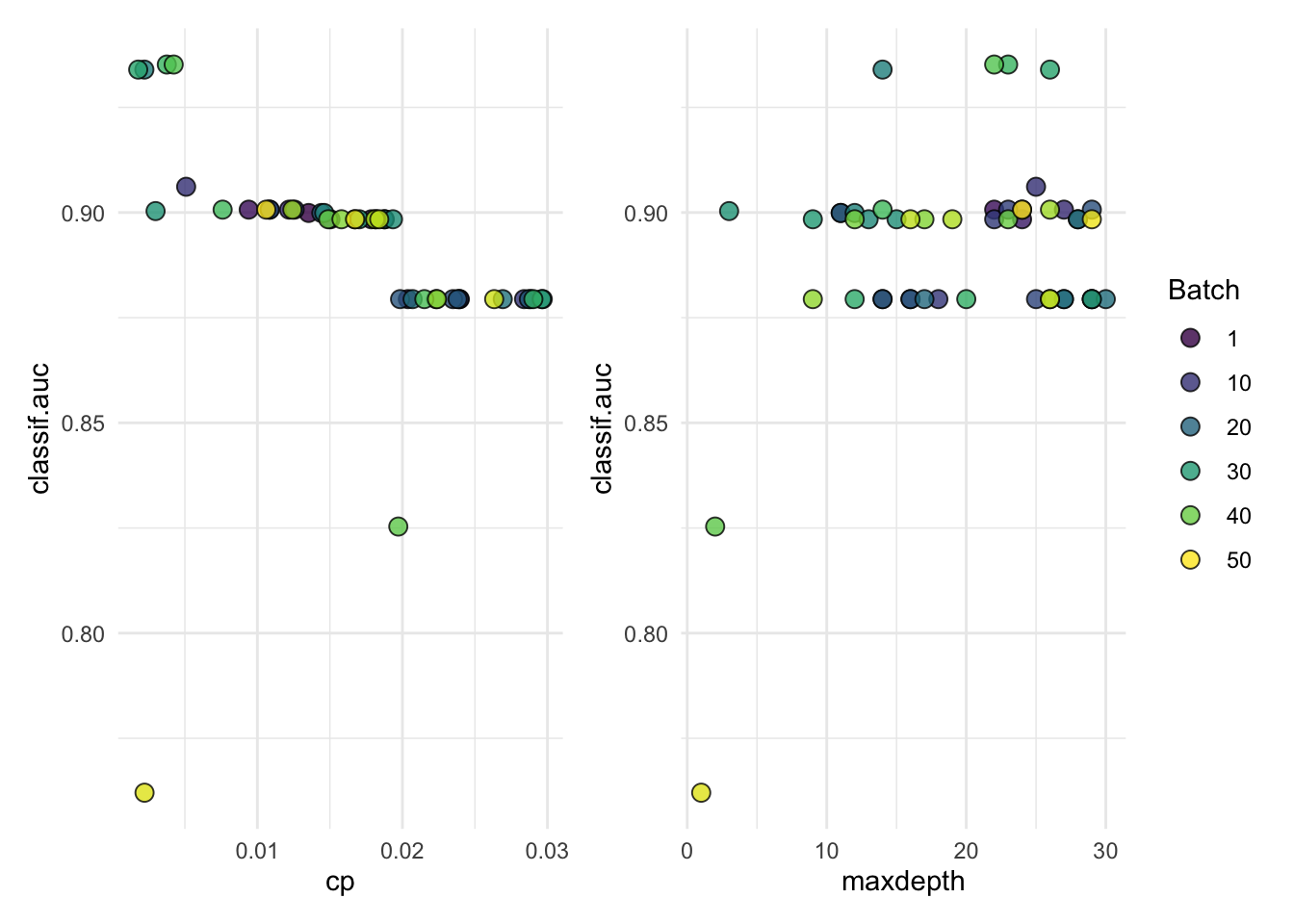

# Tuning setup
tuned_xgboost = auto_tuner(
  learner = lrn("classif.xgboost", predict_type = "prob"),
  resampling = rsmp("holdout"),
  measure = msr("classif.auc"),
  search_space = ps(
    eta = p_dbl(lower = 0.001, upper = 1),
    nrounds = p_int(lower = 1, upper = 500)
  ),
  terminator = trm("evals", n_evals = 50),
  tuner = tnr("random_search")
)

# Tune!
tuned_xgboost$train(spam_task, row_ids = spam_split$train)

autoplot(tuned_xgboost$tuning_instance, cols_x = c("nrounds", "eta"))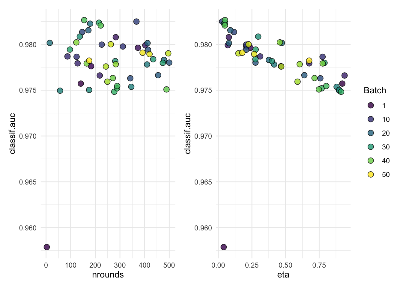

# Evaluate!
tuned_xgboost$predict(spam_task, row_ids = spam_split$test)$score(msr(
  "classif.auc"
))

#> classif.auc 
#>   0.9876319

# Tuning setup
tuned_ranger = auto_tuner(
  learner = lrn("classif.ranger", predict_type = "prob"),
  resampling = rsmp("holdout"),
  measure = msr("classif.auc"),
  search_space = ps(
    mtry.ratio = p_dbl(lower = 0, upper = 1),
    max.depth = p_int(lower = 1, upper = 30)
  ),
  terminator = trm("evals", n_evals = 50),
  tuner = tnr("random_search")
)

# Tune!
tuned_ranger$train(spam_task, row_ids = spam_split$train)

# Evaluate!
tuned_ranger$predict(spam_task, row_ids = spam_split$test)$score(msr(
  "classif.auc"
))

#> classif.auc 
#>   0.9834206

# Check parameter results
autoplot(tuned_ranger$tuning_instance)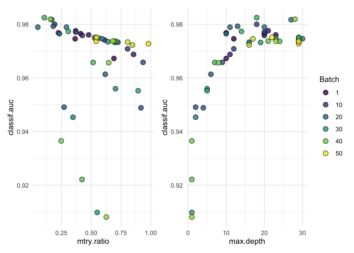

1.2 Benchmarking all the things (with tuning)

Above we tuned all the learners individually, but often we want to tune all of them at the same time to determine which performs best overall. For that, we use benchmark_grid() again (like in the second notebook), but now we just give it the AutoTuner-style learners instead of the “normal” learners.

Since we have already set up the tuning-ready learners (tuned_<method> objects) above we just recycle them here, but we first reset all of them since we already tuned them and we want to start from scratch.

tuned_knn$reset()
tuned_rpart$reset()
tuned_ranger$reset()
tuned_xgboost$reset()

tuning_learners <- list(
  tuned_knn,
  tuned_rpart,
  tuned_ranger,
  tuned_xgboost
)

tuning_benchmark_design <- benchmark_grid(
  tasks = spam_task, # Still the same task. Optional: Use list() of multiple tasks for large benchmark study
  learners = tuning_learners, # List of AutoTune-learners
  resamplings = rsmp("holdout") # Outer resampling strategy, holdout to keep it simpel
)

# Run the benchmark and save the results
future::plan("multisession", workers = 4)
bmr <- benchmark(tuning_benchmark_design)

#> Growing trees.. Progress: 28%. Estimated remaining time: 25 minutes, 3 seconds.

# Who won?
bmr$aggregate(msr("classif.auc"))

#>       nr task_id            learner_id resampling_id iters classif.auc
#>    <int>  <char>                <char>        <char> <int>       <num>
#> 1:     1    spam    classif.kknn.tuned       holdout     1   0.9607047
#> 2:     2    spam   classif.rpart.tuned       holdout     1   0.9405357
#> 3:     3    spam  classif.ranger.tuned       holdout     1   0.9803224
#> 4:     4    spam classif.xgboost.tuned       holdout     1   0.9823780
#> Hidden columns: resample_result

For statistical tests on benchmark results, refer to the mlr3benchmark package (not included with mlr3verse).

Not sure what to tune?

Which parameter to tune in which interval is usually an area of research, unless you have specific theory- or domain-driven constraints.

The mlr3tuningspaces packages aims to collect comprehensive tuning spaces for many learners, and when in doubt, they are usually a good place to start. Note that it’s most likely not necessary to extensively tune all parameters as much as possible — diminishing returns and such!