library(mlr3verse) # All the mlr3 things
library(ggplot2) # For plotting
# Silence output during tuning, mostly for cleaner output on the website
lgr::get_logger("mlr3")$set_threshold("error")

# Spam Task setup
spam_task <- tsk("spam")
set.seed(26)

# train/test split
spam_split <- partition(spam_task, ratio = 2 / 3)SVMs and more tuning
Goals of this part:
- Introduce SVMs
- Tune an SVM with a more complex setup
1 Support Vector Machines
Let’s circle back to new learners and explore SVMs a little by trying out different kernels at the example of our penguin dataset we used in the beginning:
penguins <- na.omit(palmerpenguins::penguins)

ggplot(penguins, aes(x = flipper_length_mm, y = body_mass_g, color = species)) +
  geom_point() +
  labs(
    title = "Palmer Penguins",
    x = "Flipper Length [mm]",
    y = "Body Mass [g]",
    color = "Species"
  ) +
  theme_minimal()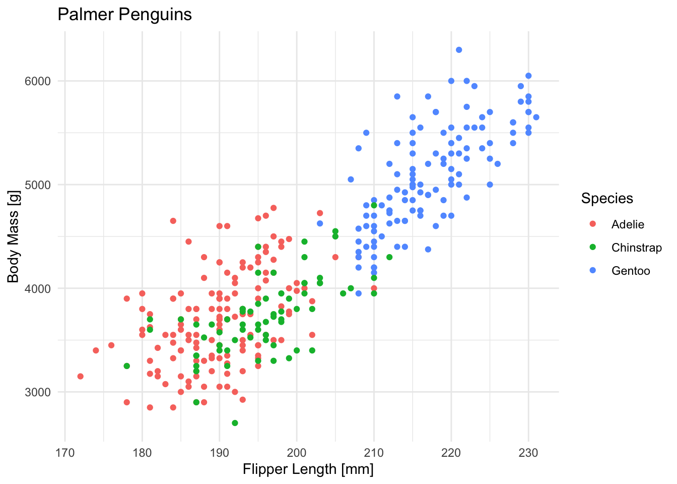
Since we don’t care about prediction accuracy for now, we’ll use the whole dataset for training and prediction. Please only do this with toy data 🙃.
For the SVM algorithm itself, we use the svm learner from the {e1071} package (great name, I know) but once again use {mlr3}’s interface
According to the docs (?e1071::svm) we have the choice of the following kernels:
"linear": \(u'v\)"polynomial": \((\mathtt{gamma} \cdot u' \cdot v + \mathtt{coef0})^\mathtt{degree}\)"radial": \(\exp(-\mathtt{gamma} \cdot |u-v|^2)\)"sigmoid": \(\tanh(\mathtt{gamma} \cdot u'v + \mathtt{coef0})\)
Where gamma, degree, and coef0 are further hyperparameters.
svm_learner <- lrn("classif.svm")

# What parameters do we have and what's the default kernel?
svm_learner$param_set
#> <ParamSet(16)>
#> Key: <id>
#> id class lower upper nlevels default parents
#> <char> <char> <num> <num> <num> <list> <list>
#> 1: cachesize ParamDbl -Inf Inf Inf 40 [NULL]
#> 2: class.weights ParamUty NA NA Inf [NULL] [NULL]
#> 3: coef0 ParamDbl -Inf Inf Inf 0 kernel
#> 4: cost ParamDbl 0 Inf Inf 1 type
#> 5: cross ParamInt 0 Inf Inf 0 [NULL]
#> 6: decision.values ParamLgl NA NA 2 FALSE [NULL]
#> 7: degree ParamInt 1 Inf Inf 3 kernel
#> 8: epsilon ParamDbl 0 Inf Inf 0.1 [NULL]
#> 9: fitted ParamLgl NA NA 2 TRUE [NULL]
#> 10: gamma ParamDbl 0 Inf Inf <NoDefault[0]> kernel
#> 11: kernel ParamFct NA NA 4 radial [NULL]
#> 12: nu ParamDbl -Inf Inf Inf 0.5 type
#> 13: scale ParamUty NA NA Inf TRUE [NULL]
#> 14: shrinking ParamLgl NA NA 2 TRUE [NULL]
#> 15: tolerance ParamDbl 0 Inf Inf 0.001 [NULL]
#> 16: type ParamFct NA NA 2 C-classification [NULL]
#> value
#> <list>
#> 1: [NULL]
#> 2: [NULL]
#> 3: [NULL]
#> 4: [NULL]
#> 5: [NULL]
#> 6: [NULL]
#> 7: [NULL]
#> 8: [NULL]
#> 9: [NULL]
#> 10: [NULL]
#> 11: [NULL]
#> 12: [NULL]
#> 13: [NULL]
#> 14: [NULL]
#> 15: [NULL]
#> 16: [NULL]1.1 Your Turn!
Below you have a boilerplate for
- Creating an SVM learner and train it on the penguin dataset with 2 predictors
- Plotting decision boundaries with it (using the
{mlr3}helper function)
Run the code below once to see what linear decision boundaries look like, then pick different kernels from the list above and run it again.
- What kernel would you pick just by the looks of the boundaries?
- How do the boundaries change if you also adjust the other hyperparameters?
- Try picking any other two variables as features (
penguin_task$col_info)
penguin_task <- as_task_classif(
  na.omit(palmerpenguins::penguins),
  target = "species"
)
penguin_task$col_roles$feature <- c("body_mass_g", "flipper_length_mm")
# Create the learner, picking a kernel and/or other hyperparams
svm_learner <- lrn("classif.svm", kernel = "polynomial", degree = 3)
# Plot decision boundaries
plot_learner_prediction(
learner = svm_learner,
task = penguin_task
)#> Warning: Raster pixels are placed at uneven horizontal intervals and will be shifted
#> ℹ Consider using `geom_tile()` instead.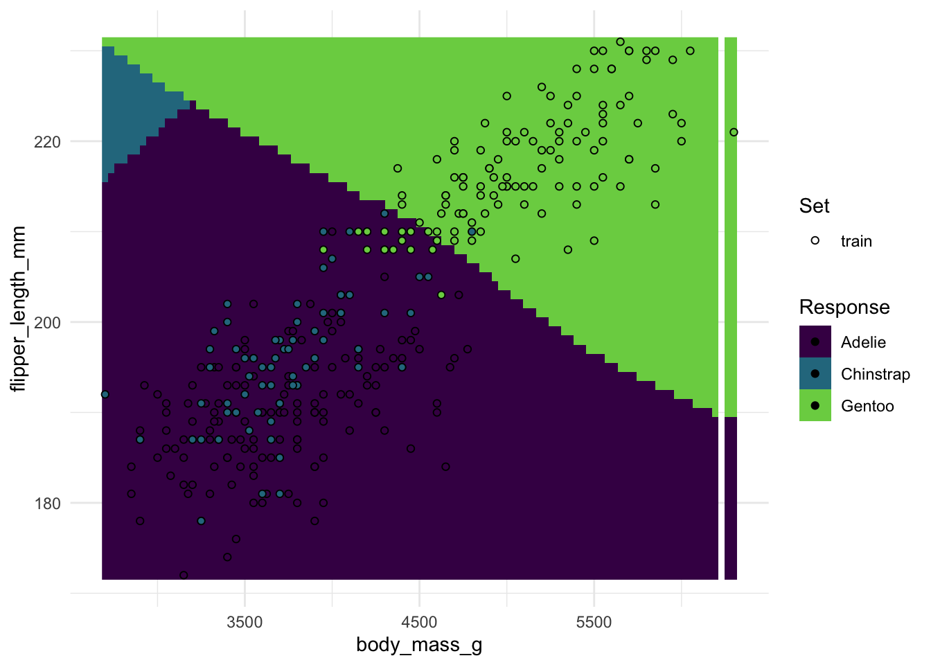
# your code
Example solution
Directly comparing multiple kernels with default parameters:
penguin_task <- as_task_classif(
  na.omit(palmerpenguins::penguins),
  target = "species"
)
penguin_task$col_roles$feature <- c("body_mass_g", "flipper_length_mm")

# Create a list of plots for each kernel
plots <- lapply(c("linear", "polynomial", "radial", "sigmoid"), \(kernel) {
  plot_learner_prediction(
    learner = lrn("classif.svm", kernel = kernel),
    task = penguin_task
  ) +
    labs(subtitle = paste("SVM with ", kernel, "kernel"))
})

# Arrange the plots with the patchwork package
patchwork::wrap_plots(plots, guides = "collect")
#> Warning: Raster pixels are placed at uneven horizontal intervals and will be shifted
#> ℹ Consider using `geom_tile()` instead.
#> Raster pixels are placed at uneven horizontal intervals and will be shifted
#> ℹ Consider using `geom_tile()` instead.
#> Raster pixels are placed at uneven horizontal intervals and will be shifted
#> ℹ Consider using `geom_tile()` instead.
#> Raster pixels are placed at uneven horizontal intervals and will be shifted
#> ℹ Consider using `geom_tile()` instead.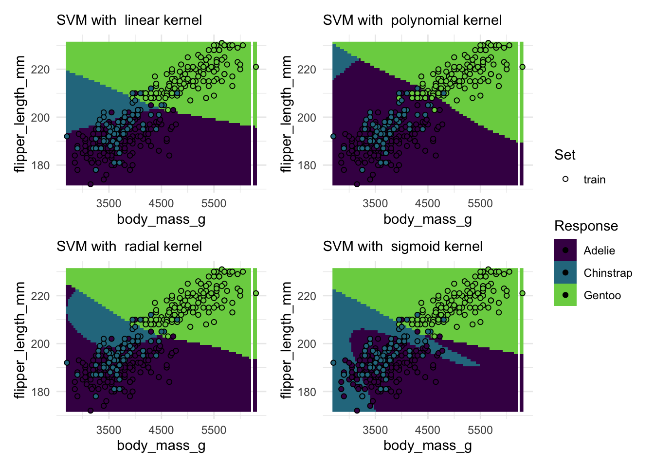
1.2 SVM-Tuning
Let’s try a more complex tuning experiment, based on the spam task from before.
We’ll create a new SVM learner object and this time explicitly tell it which classification to do — that’s the default value anyway, but {mlr3} wants us to be explicit here for tuning:
svm_learner <- lrn(
  "classif.svm",
  predict_type = "prob",
  type = "C-classification"
)
First up we’ll define our search space, meaning the range of parameters we want to test out. Since kernel is a categorical parameter (i.e. no numbers, just names of kernels), we’ll define the search space for that parameter by just passing the names of the kernels to the p_fct() helper function that defines factor-parameters in {mlr3}.
The interesting thing here is that some parameters are only relevant for some kernels, which we can declare via a depends argument:
search_space_svm = ps(
  kernel = p_fct(c("linear", "polynomial", "radial", "sigmoid")),
  # Degree is only relevant if "kernel" is "polynomial"
  degree = p_int(lower = 1, upper = 7, depends = kernel == "polynomial")
)
We can create an example design grid to inspect our setup and see that degree is NA for cases where kernel is not "polynomial", just as we expected
generate_design_grid(search_space_svm, resolution = 3)#> <Design> with 6 rows:
#> kernel degree
#> <char> <int>
#> 1: linear NA
#> 2: polynomial 1
#> 3: polynomial 4
#> 4: polynomial 7
#> 5: radial NA
#> 6: sigmoid NA1.3 Your Turn!
The above should get you started to…
- Create a
search_space_svmlike above, tuning…
costfrom 0.1 to 1 (hint:logscale = TRUEor e.g.trafo = function(x) 10^x)kernel, (like above example)degree, as above, only ifkernel == "polynomial"gamma, from e.g. 0.01 to 0.2, only ifkernelis polynomial, radial, sigmoid (hint: you can’t usekernel != "linear"unfortunately, butkernel %in% c(...)) works
- Use the
auto_tunerfunction as previously seen with
svm_learner(see above)- A resampling strategy (use
"holdout"if runtime is an issue) - A measure (e.g.
classif.accorclassif.auc) - The search space you created in 1.
- A termination criterion (e.g. 40 evaluations)
- Random search as your tuning strategy
- Train the auto-tuned learner and evaluate on the test set
What parameter settings worked best?
# your code
Example solution
search_space_svm = ps(
  cost = p_dbl(-1, 1, trafo = function(x) 10^x),
  kernel = p_fct(c("linear", "polynomial", "radial", "sigmoid")),
  degree = p_int(1, 7, depends = kernel == "polynomial"),
  gamma = p_dbl(
    lower = 0.01,
    upper = 0.2,
    depends = kernel %in% c("polynomial", "radial", "sigmoid")
  )
)

grid <- generate_design_grid(search_space_svm, resolution = 6)

# Look at grid with transformed cost param (manual way, there's probably a better one)
grid$data$cost_trafo <- 10^grid$data$cost
grid$data
#> cost kernel degree gamma cost_trafo
#> <num> <char> <int> <num> <num>
#> 1: -1 linear NA NA 0.1
#> 2: -1 polynomial 1 0.010 0.1
#> 3: -1 polynomial 1 0.048 0.1
#> 4: -1 polynomial 1 0.086 0.1
#> 5: -1 polynomial 1 0.124 0.1
#> ---
#> 290: 1 sigmoid NA 0.048 10.0
#> 291: 1 sigmoid NA 0.086 10.0
#> 292: 1 sigmoid NA 0.124 10.0
#> 293: 1 sigmoid NA 0.162 10.0
#> 294: 1 sigmoid NA 0.200 10.0set.seed(313)
tuned_svm = auto_tuner(
learner = lrn(
"classif.svm",
predict_type = "prob",
type = "C-classification"
),
resampling = rsmp("holdout"),
measure = msr("classif.auc"),
search_space = search_space_svm,
terminator = trm("evals", n_evals = 40),
tuner = tnr("random_search")
)
# Tune!
tuned_svm$train(spam_task, row_ids = spam_split$train)
# Evaluate!
tuned_svm$predict(spam_task, row_ids = spam_split$test)$score(msr(
"classif.auc"
))#> classif.auc
#> 0.9702688# Hyperparam winner:
tuned_svm$tuning_result#> cost kernel degree gamma learner_param_vals x_domain classif.auc
#> <num> <char> <int> <num> <list> <list> <num>
#> 1: -0.5680516 linear NA NA <list[3]> <list[2]> 0.9692524# Remember that we transformed `cost`, here's the best value on the original scale
tuned_svm$tuning_result$x_domain#> [[1]]
#> [[1]]$cost
#> [1] 0.2703637
#>
#> [[1]]$kernel
#> [1] "linear"autoplot(tuned_svm$tuning_instance)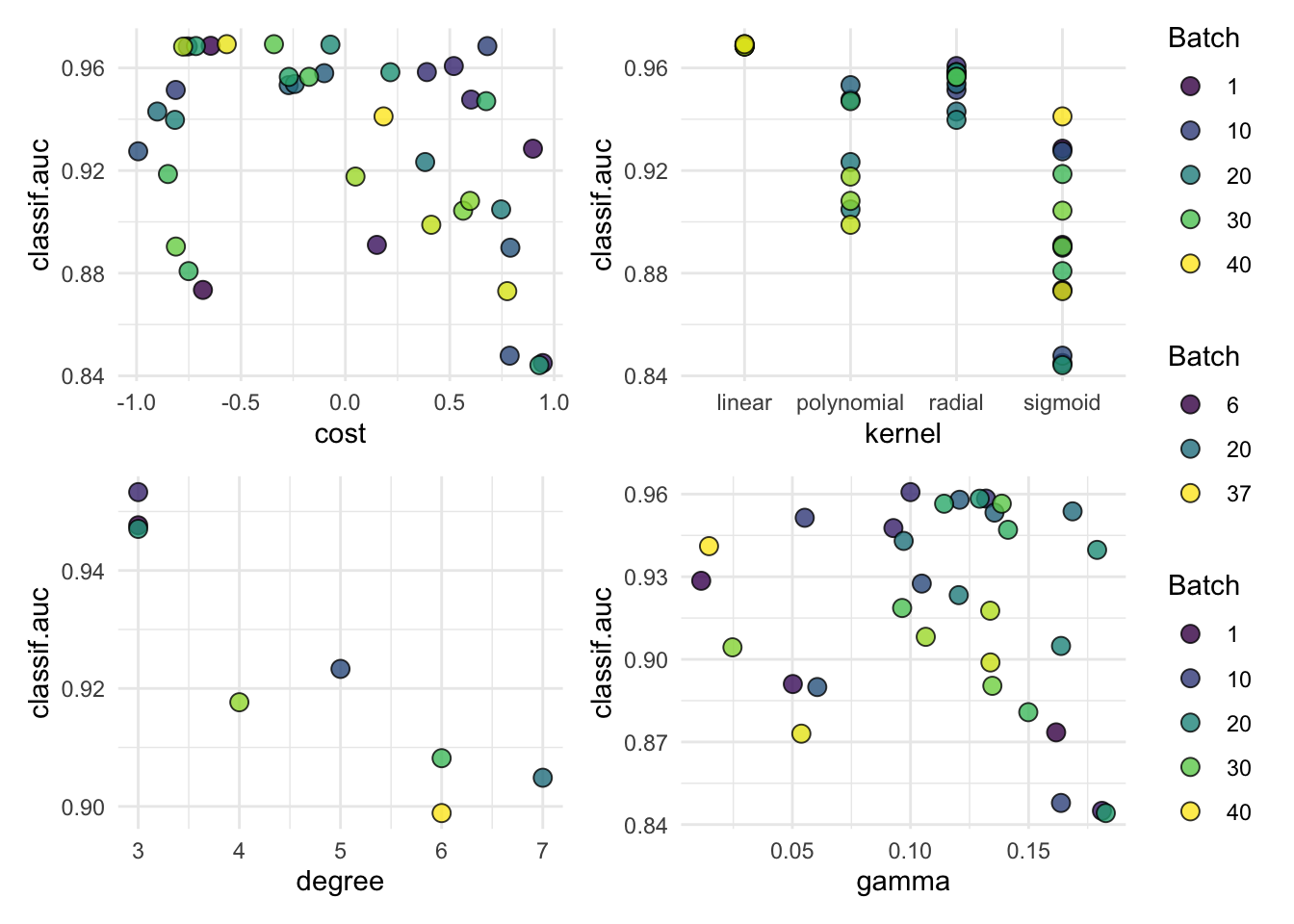
Since the penguins data is a bit different we need to make a few tweaks to our setup:
- The AUC is only defined for binary classification targets, and while there are different versions of the AUC suitable for multiclass prediction, we just switch to the classification error as our tuning metric
- The data has categorical features, such as
island. We dummy- (or treatment-) encode our data using the"encode"PipeOp (see docs at?mlr3pipelines:::PipeOpEncode). - Because we add a PipeOp to the learner, we need to prefix its parameters in the search space definition with its ID, which we also assign. That ID used to be
classif.svm, but giving it a short name is convenient. This is an easy to overlook detail in a live workshop setting cough.
# Penguin task setup
penguin_task = as_task_classif(
  na.omit(palmerpenguins::penguins),
  target = "species"
)
penguin_splits = partition(penguin_task)
base_svm = po("encode") %>>%
po(
"learner",
lrn(
"classif.svm",
predict_type = "prob",
type = "C-classification",
id = "svm" # give it an ID to identify its parameters more easily
)
) |>
as_learner()In the parameter search space we need to prefix the parameters for the SVM with it’s ID we set above, because technically other preprocessing pipeline parameters could also have parameters to tune, such and the "encode" PipeOp where we could technically tune "method" in c("treatment", "one-hot", "helmert", "poly", "sum") if we wanted to compare different methods of encoding categorical features. In this case though there’s not really any point, because dummy (here “treatment”) encoding is the default methid and is usually fine, and one-hot is the only alternative we might care about.
tuned_svm = auto_tuner(
  learner = base_svm,
  resampling = rsmp("holdout"),
  measure = msr("classif.ce"),
  search_space = ps(
    svm.cost = p_dbl(-1, 1, trafo = function(x) 10^x),
    svm.kernel = p_fct(c("linear", "polynomial", "radial", "sigmoid")),
    svm.degree = p_int(1, 7, depends = svm.kernel == "polynomial"),
    svm.gamma = p_dbl(
      lower = 0.01,
      upper = 0.2,
      depends = svm.kernel %in% c("polynomial", "radial", "sigmoid")
    )
  ),
  terminator = trm("evals", n_evals = 100),
  tuner = tnr("random_search")
)

# Tune!
tuned_svm$train(penguin_task, row_ids = penguin_splits$train)
tuned_svm$tuning_result
#> svm.cost svm.kernel svm.degree svm.gamma learner_param_vals x_domain
#> <num> <char> <int> <num> <list> <list>
#> 1: -0.4159897 linear NA NA <list[4]> <list[2]>
#> classif.ce
#> <num>
#> 1: 0# Predict and evaluate
svm_preds = tuned_svm$predict(penguin_task, row_ids = penguin_splits$test)
svm_preds$score(msr("classif.acc"))#> classif.acc
#> 1# Remember that we transformed `cost`, here's the best value on the original scale
tuned_svm$tuning_result$x_domain[[1]]$svm.cost#> [1] 0.3837163autoplot(tuned_svm$tuning_instance)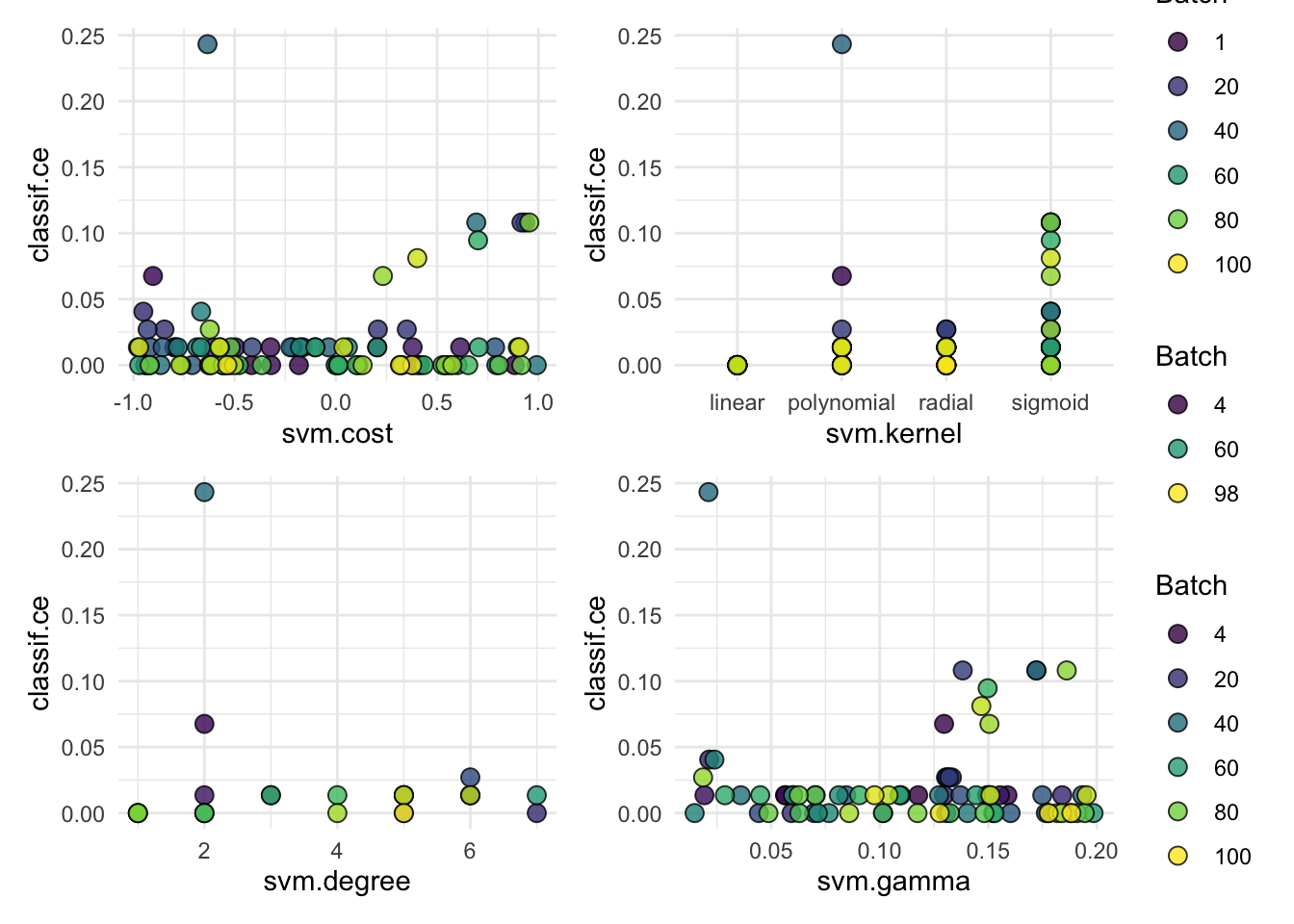
SVM with categorical features
We have not covered this so far, but if you want to tran an SVM (or many other learners) on tasks with categorical (“nominal”) features (usually factor in R), we first need to encode them in a numeric format. The simplest way is to perform dummy- or one-hot encoding, and mlr3 has a whole slew of these sorts of rpeprocessing capabilities.
This works by creating a pipeline using the %>>% oeprator (not to be confused with the magrittr-pipe %>% you might be familiar with!). We take the encode pipeline operation (PipeOp) and stack it on top of our learner we create as usual. At the end we convert it to a regular learner, and lrn_svm is now a regular mlr3 learner we can use like any other, but with built-in encoding!
lrn_svm_base <- lrn("classif.svm", predict_type = "prob")

lrn_svm <- po("encode") %>>%
  po("learner", lrn_svm_base) |>
  as_learner()

# Penguin task (including categoricals!)
penguin_task <- as_task_classif(
  na.omit(palmerpenguins::penguins),
  target = "species"
)

# Quick demo
lrn_svm$train(penguin_task)
lrn_svm$predict(penguin_task)
#>
#> ── <PredictionClassif> for 333 observations: ───────────────────────────────────
#> row_ids truth response prob.Adelie prob.Chinstrap prob.Gentoo
#> 1 Adelie Adelie 0.9902015480 0.004221288 0.005577164
#> 2 Adelie Adelie 0.9809077769 0.009140092 0.009952131
#> 3 Adelie Adelie 0.9774767198 0.012267394 0.010255886
#> --- --- --- --- --- ---
#> 331 Chinstrap Chinstrap 0.0162354405 0.976858790 0.006905770
#> 332 Chinstrap Chinstrap 0.0061838595 0.985258938 0.008557203
#> 333 Chinstrap Chinstrap 0.0006315615 0.992851159 0.006517280Pipelines are extremely useful and part of any reasonably complex machine learning pipeline, and to learn more you can read the chapter in the mlr3book.
Note that PipeOps can have their own parameters, which could also be subject to tuning!