Example on Real Multi-modal Medical Data • survinng

This vignette demonstrates how to apply gradient-based attribution methods to a multi-modal survival model trained on real medical data. Specifically, we explore the interpretability of a DeepHit-style neural network that jointly processes tabular and image-based features. The model is evaluated on a set of test instances and visualized using various attribution techniques.

Note: Since the images used in this example are of size (3, 226, 226), running this example may take a while or too much memory, especially for the GradSHAP(t) and IntGrad(t) methods if too many samples are used. To avoid this, we recommend using smaller sample sizes or number of integration points.

Setup

We begin by loading the necessary libraries and setting the seeds to ensure reproducibility. The helper functions used for image processing and visualization are sourced from a separate utility script which can be found in the vignettes/articles/real_data directory or online in the GitHub repository.

library(survinng)
library(torch)
library(torchvision)
library(ggplot2)
library(data.table)
library(cowplot)
library(dplyr)
library(here)

# Load helper functions
source(here("vignettes/articles/real_data/utils.R"))

# Set seeds for reproducibility
set.seed(42)
torch_manual_seed(42)

Load model and metadata

We first load the trained model along with its corresponding metadata, including the number of outputs for the image and joint components, whether a bias term was included, and the number of tabular features. The model’s performance is briefly summarized using two commonly used survival metrics: the Concordance index and the Integrated Brier Score.

After restoring the model’s state dictionary, we replicate the multi-modal network structure consisting of a ResNet34 backbone for the image branch and a linear transformation for the tabular input.

All required files are available in the vignettes/articles/real_data directory or online in the GitHub repository folder.

# Load model metadata
model_metadata <- read.csv(here("vignettes/articles/real_data/metadata.csv"))
n_img_out <- model_metadata$n_img_out
n_out <- model_metadata$n_out
out_bias <- as.logical(model_metadata$out_bias)
n_tab_feat <- model_metadata$Number.of.tabular.features

# Show performance results
model_metadata[, c("Concordance", "Integrated.Brier.score")]
#>   Concordance Integrated.Brier.score
#> 1   0.7133996              0.0919935

# Load model state dict
model_state_dict <- load_state_dict(here("vignettes/articles/real_data/model.pt"))

# Replicate model
net_image <- torchvision::model_resnet34(num_classes = n_img_out)
model <- MultiModalModel(net_image, tabular_features = rep(1, n_tab_feat),
                         n_out = n_out, n_img_out = n_img_out, out_bias = out_bias)

# Load model state dict
model <- model$load_state_dict(model_state_dict)
model$eval()
model
#> An `nn_module` containing 21,518,292 parameters.
#> 
#> ── Modules ─────────────────────────────────────────────────────────────────────
#> • net_images: <resnet> #21,416,000 parameters
#> • fc1: <nn_linear> #66,816 parameters
#> • fc2: <nn_linear> #32,896 parameters
#> • relu: <nn_relu> #0 parameters
#> • drop_0_3: <nn_dropout> #0 parameters
#> • drop_0_4: <nn_dropout> #0 parameters
#> • out: <nn_linear> #2,580 parameters

Load data

Next, we prepare the input data for evaluation and explanation. This includes:

A tabular dataset containing numeric predictors.
Corresponding image files from the test set.

Images are preprocessed using standard transformations (center cropping and normalization) and stacked into a single tensor. The tabular inputs are converted into a Torch tensor to be compatible with the model input format.

Note: The tabular and image data can be found in the vignettes/articles/real_data directory or online in the GitHub repository folder.

data <- read.csv(here("vignettes/articles/real_data/deephit_tabular_data.csv"))
test_images <- list.files(here("vignettes/articles/real_data/test"), full.names = FALSE)

# Filter data
data <- data[data$full_path %in% test_images, ]
data_tab <- torch_tensor(as.matrix(data[, c(1, 2, 3, 4)]))
data_img <- torch_stack(lapply(data$full_path, function(x) {
  base_loader(here(paste0("vignettes/articles/real_data/test/", x))) %>%
    (function(x) x[,,1:3]) %>%
    transform_to_tensor() %>%
    transform_center_crop(226) %>%
    transform_normalize(mean = c(0.485, 0.456, 0.406), std = c(0.229, 0.224, 0.225))
}), dim = 1)

Explain model

We apply several gradient-based feature attribution techniques adapted for survival analysis to explain the model’s prediction of a selected test instance:

Grad(t): Simple backpropagation-based gradients with respect to the input.
SG(t): A noise-averaged version of gradients to improve local fluctuations of the gradients.
IG(t): A path-based method that accumulates gradients along a linear interpolation between a baseline and the input. In this example, we use a mean baseline.
GradSHAP(t): An approximation to SHAP values using randomized baseline samples combined with gradient integration.

Each method runs with a moderate batch size of 10 and a fixed number of samples to ensure computational feasibility. For better estimates, we recommend using larger sample sizes or number of integration points, but this may lead to increased memory usage and longer computation times. The explanations are stored in data.tables for downstream visualization.

exp_deephit <- survinng::explain(model, list(data_img, data_tab), 
                                 model_type = "deephit",
                                 time_bins = seq(0, 17, length.out = n_out))

ids <- 230
orig_img <- base_loader(here(paste0("vignettes/articles/real_data/test/", data[ids, ]$full_path)))

# Run Grad(t)
grad <- surv_grad(exp_deephit, instance = ids, batch_size = 10)
gc()

# Run SG(t)
sgrad <- surv_smoothgrad(exp_deephit, instance = ids, n = 50, 
                         noise_level = 0.3, batch_size = 10)
gc()

# Run IntGrad(t)
intgrad <- surv_intgrad(exp_deephit, instance = ids, n = 50, batch_size = 10) 
gc()

# Run GradSHAP(t)
grad_shap <- surv_gradSHAP(exp_deephit, instance = ids, n = 10, num_samples = 50, 
                           batch_size = 10, replace = FALSE) 
gc()

# Convert to data.tables
grad <- as.data.table(grad)
sgrad <- as.data.table(sgrad)
intgrad <- as.data.table(intgrad)
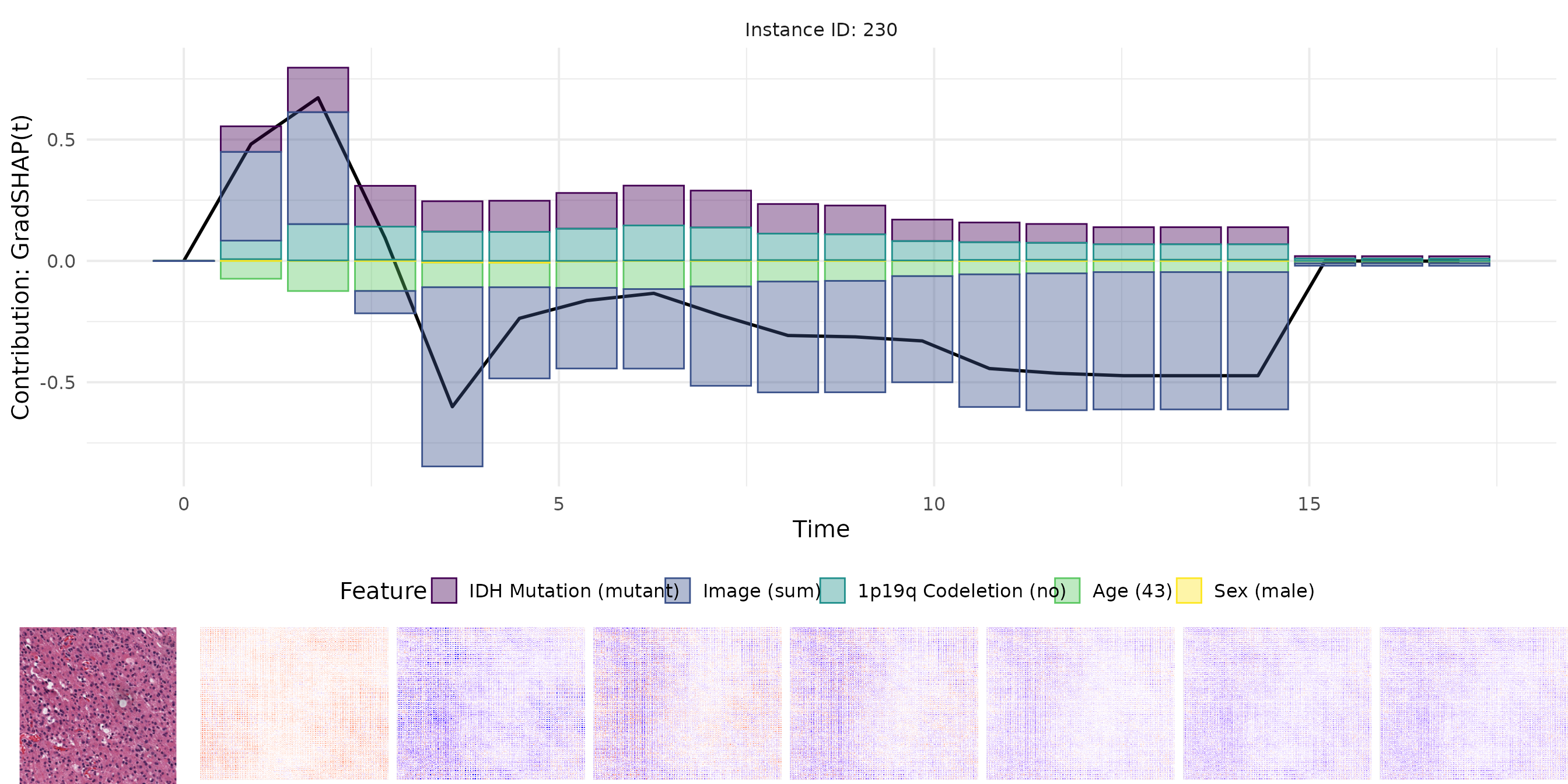
grad_shap <- as.data.table(grad_shap)

Visualize results

For each method, we visualize:

The original image.
The pixel-wise relevance heatmap.
A combined view aligning tabular and image attributions.

The plots enable a comparative interpretation of how each attribution method highlights relevant regions in the image and important features in the tabular input over time. In particular, the visualizations allow us to examine the consistency and plausibility of attributions across methods, offering insight into the internal reasoning of the survival model.

Plot Grad(t)

plots <- plot_result(grad, orig_img, name = "real_data_grad", as_force = FALSE)
plot_grid(plots[[1]], 
          plot_grid(plots[[3]], plots[[2]], nrow = 1, rel_widths = c(1, 7)),
          rel_heights = c(1, 0.25), nrow = 2)

Plot SG(t)

plots <- plot_result(sgrad, orig_img, name = "real_data_sgrad", as_force = FALSE)
plot_grid(plots[[1]], 
          plot_grid(plots[[3]], plots[[2]], nrow = 1, rel_widths = c(1, 7)),
          rel_heights = c(1, 0.25), nrow = 2)

Plot IntGrad(t)

plots <- plot_result(intgrad, orig_img, name = "real_data_intgrad", as_force = TRUE)
plot_grid(plots[[4]], 
          plot_grid(plots[[3]], plots[[2]], nrow = 1, rel_widths = c(1, 7)),
          rel_heights = c(1, 0.25), nrow = 2)

Plot GradSHAP(t)

plots <- plot_result(grad_shap, orig_img, name = "real_data_gradshap", as_force = TRUE)
plot_grid(plots[[4]], 
          plot_grid(plots[[3]], plots[[2]], nrow = 1, rel_widths = c(1, 7)),
          rel_heights = c(1, 0.25), nrow = 2)