Simulation of Time-dependent Effects • survinng

In this vignette we simulate survival data to detect time-dependent feature effects using gradient-based explanation techniques for survival neural network models.

Load the necessary libraries and source the utility functions.

library(survinng)
library(ggplot2)
library(cowplot)
library(dplyr)
library(tidyr)
library(survival)
library(survminer)
library(torch)
library(viridis)
library(here)

# Set seed for reproducibility
set.seed(2025)
torch_manual_seed(2025)

Preprocessing

Generate the Data

We consider a simulated dataset with the following characteristics:

Sample size: 10,000 individuals
- 9,500 samples used for training
- 500 samples used for testing
Covariates:
- $X_1 \sim N(0, 1)$ : has a time-dependent effect on the hazard:
  - Initially a negative effect
  - Later transitions to a positive effect
    (This implies the opposite effect on the survival probability)
- $X_2 \sim \mathcal{N}(0, 1)$ : has a positive effect on the hazard
  → Negative effect on survival
- $X_3 \sim \mathcal{U}(0, 1)$ : has a strong negative effect on the hazard
  → Positive effect on survival
- $X_4 \sim \mathcal{U}(-1, 1)$ : has no effect on the hazard or survival

Load Models and Data

The models used in this vignette are the same as those used in the main paper. The models were trained using the survivalmodels package, and the training process is not shown here, but can be found in the vignettes/articles/Sim_time_dependent directory or on GitHub.

# Load data
train <- readRDS(here("vignettes/articles/Sim_time_dependent/train.rds"))
test <- readRDS(here("vignettes/articles/Sim_time_dependent/test.rds"))
dat <- rbind(train, test)

# Load extracted models
ext_coxtime <- readRDS(here("vignettes/articles/Sim_time_dependent/extracted_model_coxtime.rds"))
ext_deepsurv <- readRDS(here("vignettes/articles/Sim_time_dependent/extracted_model_deepsurv.rds"))
ext_deephit <- readRDS(here("vignettes/articles/Sim_time_dependent/extracted_model_deephit.rds"))

Performance

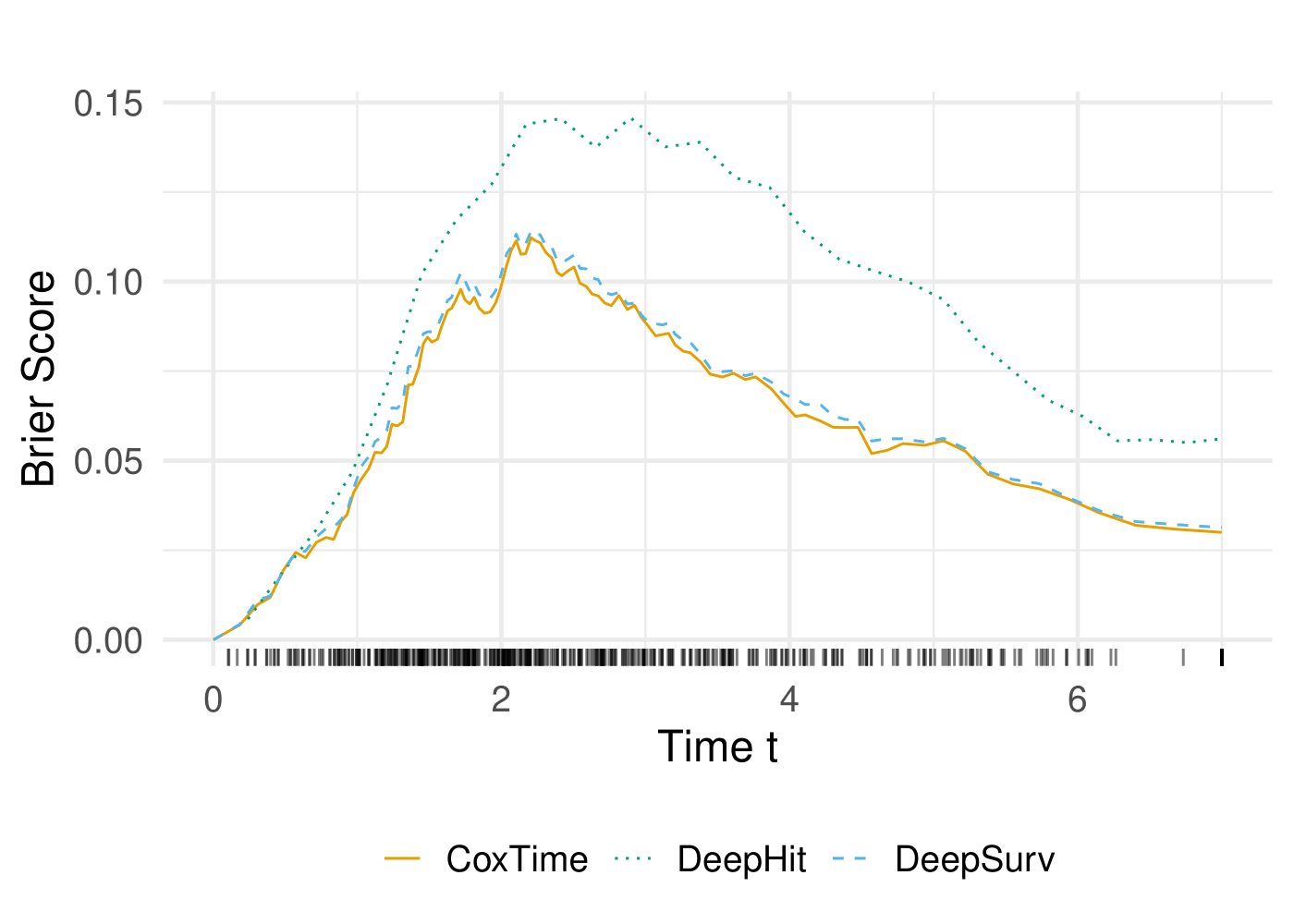
The performance of the models is evaluated using the C-Index and Integrated Brier Score (IBS). The C-Index measures the concordance between predicted and observed survival times, while the IBS quantifies the accuracy of survival predictions.

Model	C-Index	IBS
CoxTime	0.845570	0.058430
DeepSurv	0.859624	0.060411
DeepHit	0.806480	0.095961

Create Explainer

The explain() function creates an explainer object for the survival models. The data argument specifies the dataset used for explanation, and the model argument specifies the model to be explained. The target argument indicates the type of prediction to be explained (e.g., “survival”, “risk”, “cumulative hazard”).

exp_deephit <- survinng::explain(ext_deephit[[1]], data = test)
exp_coxtime <- survinng::explain(ext_coxtime[[1]], data = test)
exp_deepsurv <- survinng::explain(ext_deepsurv[[1]], data = test)

Kaplan-Meier Survival Curves

The Kaplan-Meier survival curves are plotted to visualize the survival probabilities over time. The x1 variable is categorized into two groups (low and high) based on its median value. The survival curves are then plotted for each group.

# Categorize `x1` into bins (e.g., low, medium, high)
dat$x1_group <- cut(dat$x1, 
                    breaks = quantile(dat$x1, probs = c(0, 0.5, 1)), 
                    labels = c("Low", "High"), 
                    include.lowest = TRUE)

# Create a Surv object
surv_obj <- Surv(dat$time, dat$status)

# Fit Kaplan-Meier survival curves stratified by `x1_group`
km_fit <- survfit(surv_obj ~ x1_group, data = dat)

# Plot the KM curves
km_plot <- ggsurvplot(km_fit, 
                      data = dat,
                      xlab = "Time t",
                      ylab = "Survival Probability",
                      legend.title = "x1 Group",
                      palette = c("#377EB8", "#E69F00"),  
                      title = "") 
km_plot$plot <- km_plot$plot + 
  theme_minimal(base_size = 17) +
  theme(legend.position = "bottom") +
  geom_rug(data = test, aes(x = time), sides = "bl", linewidth = 0.5, alpha = 0.5, inherit.aes = FALSE)
km_plot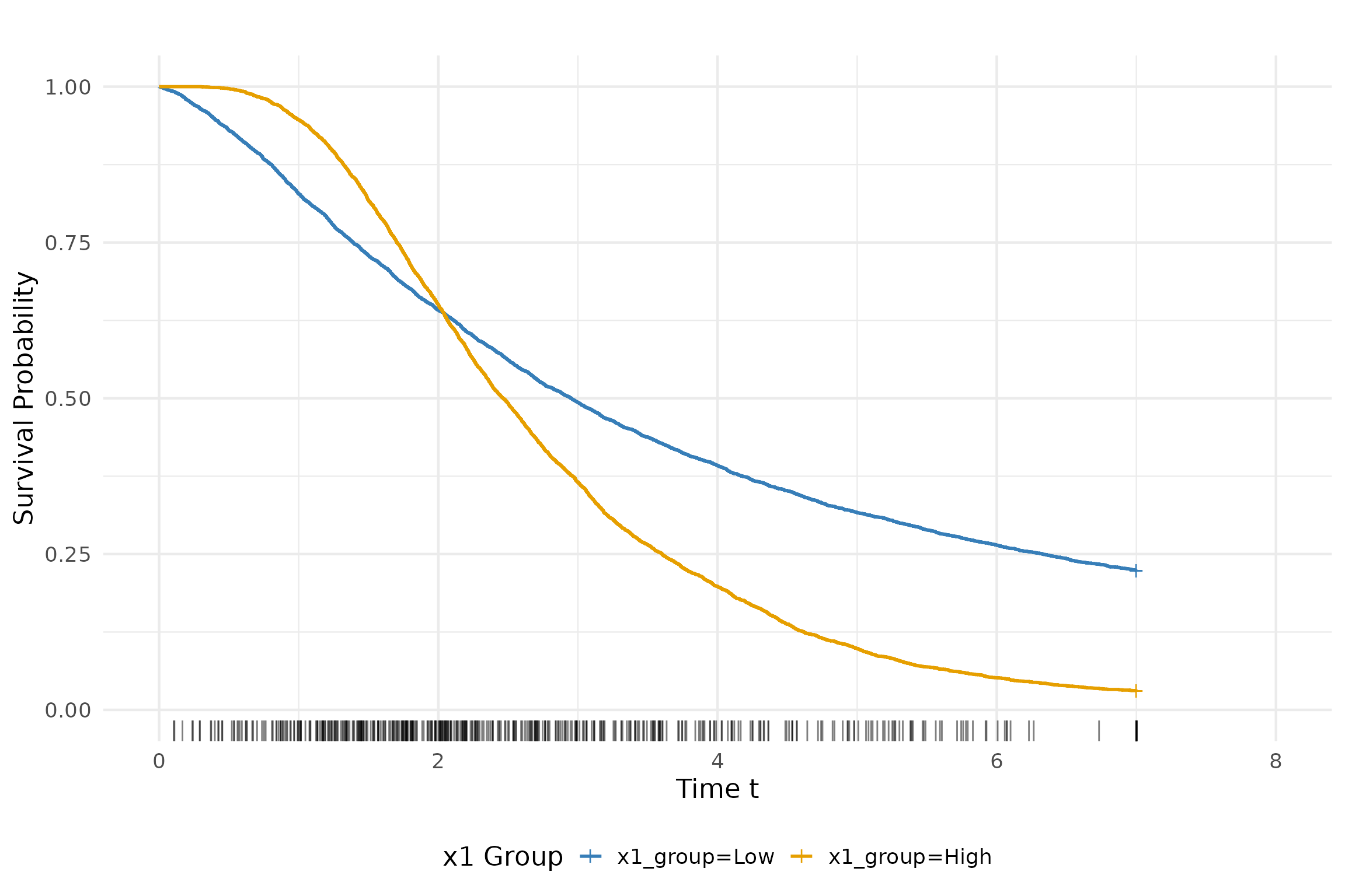

Survival Prediction

The survival predictions for the test dataset are computed using the predict() function. The type argument specifies the type of prediction to be made (e.g., “survival”, “risk”, “cumulative hazard”). The survival predictions are then plotted for a set of instances of interest.

# Print instances of interest
td_ids <- c(79, 428)
print(test[td_ids, ])
#>          time status        x1         x2         x3         x4
#> 1535 4.306154      1 0.1934749 -0.3069111 -0.1475012  0.6370386
#> 8202 1.417212      1 0.7526954 -0.3781274 -1.1500862 -0.6418508

# Compute Vanilla Gradient
grad_cox <- surv_grad(exp_coxtime, target = "survival", instance = td_ids)
grad_deephit <- surv_grad(exp_deephit, target = "survival", instance = td_ids)
grad_deepsurv <- surv_grad(exp_deepsurv, target = "survival", instance = td_ids)

# Plot survival predictions
surv_plot <- cowplot::plot_grid(
  plot(grad_cox, type = "pred") ,
  plot(grad_deephit, type = "pred"),
  plot(grad_deepsurv, type = "pred"),
  nrow = 1, labels = c("CoxTime", "DeepHit", "DeepSurv"),
  label_x = 0.03,      
  label_size = 14) 
surv_plot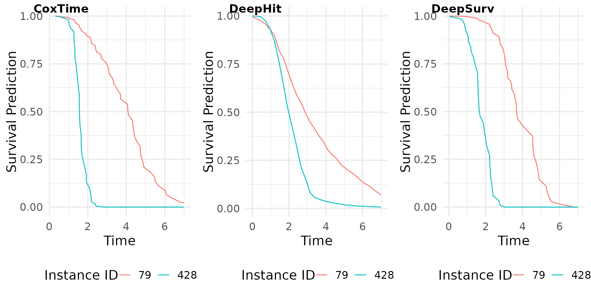

Explainable AI

The following sections demonstrate the application of various gradient-based explanation methods to the survival models. The methods include Grad(t), SmoothGrad(t), IntGrad(t), and GradSHAP(t), corresponding to the plots shown in the main body of the paper.

Grad(t) (Sensitivity)

Here we compute the gradient of the survival predictions with respect to the input features. The surv_grad() function computes the gradients for the specified instances.

# Plot attributions
grad_plot <- cowplot::plot_grid(
  plot(grad_cox, type = "attr") ,
  plot(grad_deephit, type = "attr"),
  plot(grad_deepsurv, type = "attr"),
  nrow = 3, labels = c("CoxTime", "DeepHit", "DeepSurv"))
grad_plot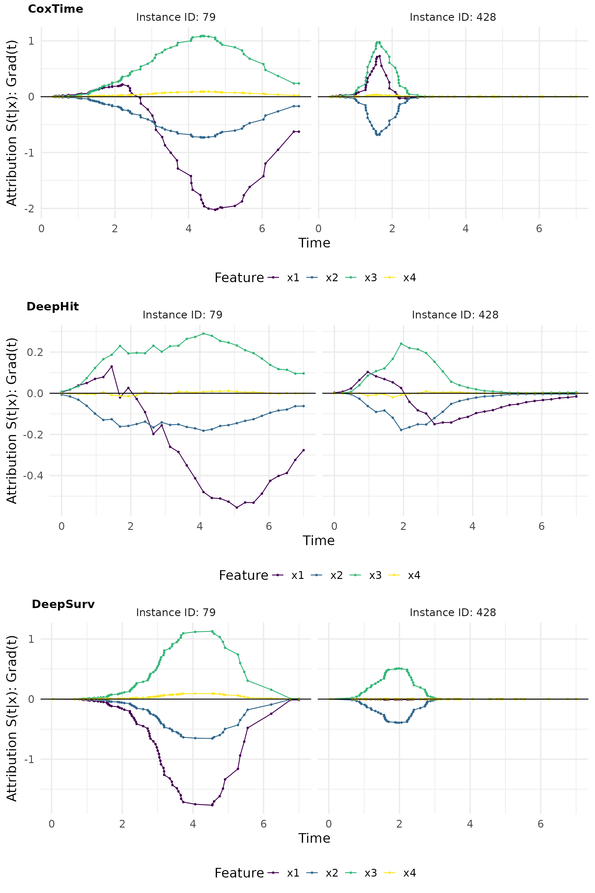

SmoothGrad(t) (Sensitivity)

SmoothGrad(t) is a method that adds noise to the input features and computes the average gradient over multiple noisy samples. This approach helps to reduce the noise in the gradient estimates and provides a clearer picture of the feature importance.

# Compute SmoothGrad
sg_cox <- surv_smoothgrad(exp_coxtime, target = "survival", instance = td_ids, 
                          n = 50, noise_level = 0.1)
sg_deephit <- surv_smoothgrad(exp_deephit, target = "survival", instance = td_ids, 
                              n = 50, noise_level = 0.1)
sg_deepsurv <- surv_smoothgrad(exp_deepsurv, target = "survival", instance = td_ids, 
                               n = 50, noise_level = 0.1)

# Plot attributions
smoothgrad_plot <- cowplot::plot_grid(
  plot(sg_cox, type = "attr"), 
  plot(sg_deephit, type = "attr"), 
  plot(sg_deepsurv, type = "attr"),
  nrow = 3, labels = c("CoxTime", "DeepHit", "DeepSurv"))
smoothgrad_plot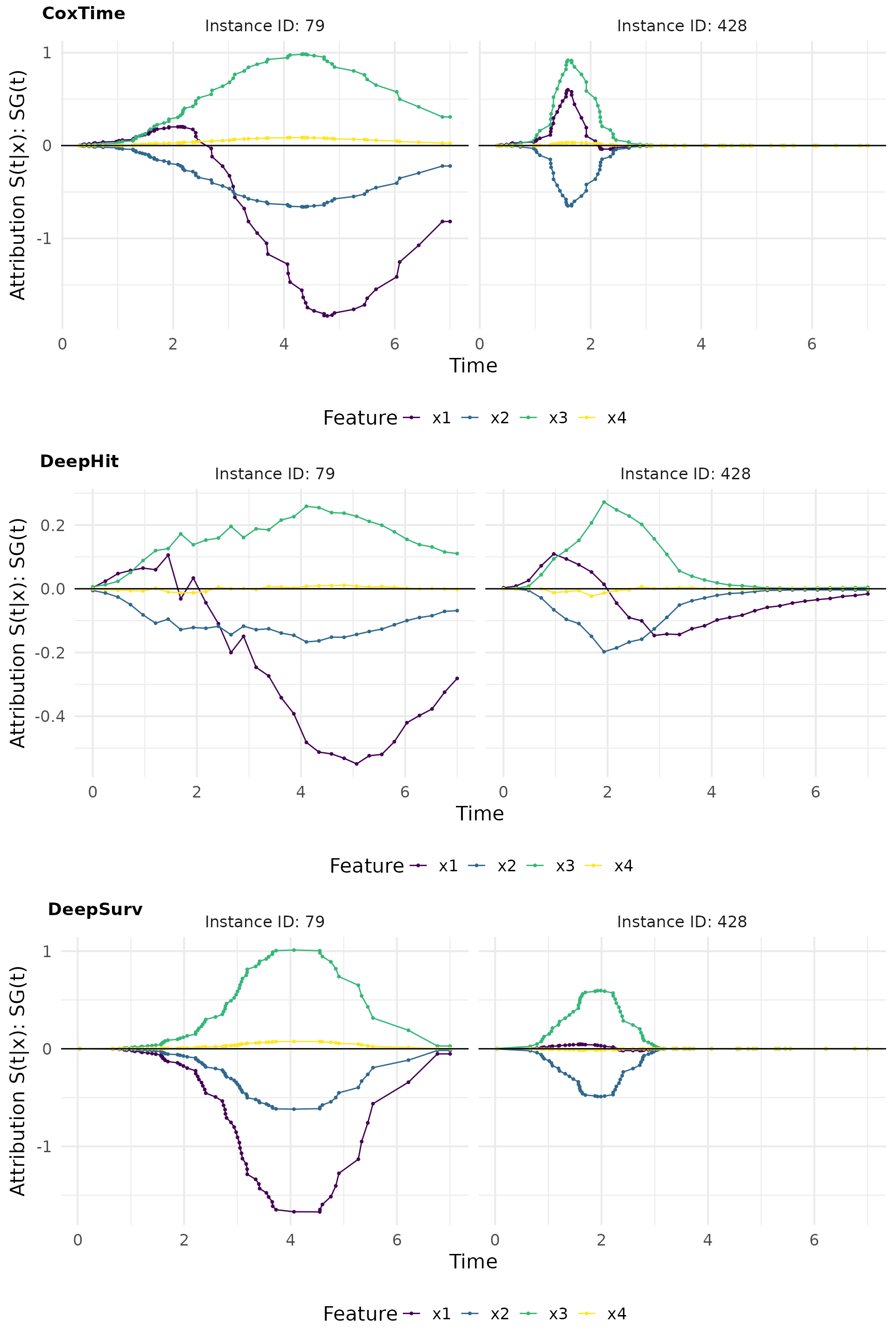

The relevance curves derived from output-sensitive methods effectively reveal the time-dependent effect of $x_1$ on the survival predictions, by indicating a positive effect at earlier times and a negative effect later on. This time-dependent effect is accurately captured by CoxTime and DeepHit, but not by DeepSurv, which is inherently constrained by the PH assumption and thus unable to model time-dependence.

IntGrad(t)

IntGrad(t) is a method that computes the integral of the gradients along a straight line path from a reference point to the input instance. This method provides a more comprehensive view of the feature importance by considering the cumulative effect of the features over time.

In addition to time-dependence in feature effects, difference-to-reference methods (i.e., IntGrad(t) and GradSHAP(t)) provide insights into the relative scale, direction, and magnitude of feature effects by comparing predictions to a meaningful reference.

Zero baseline

The zero baseline is a reference point where all features are set to zero.

# Compute IntegratedGradient with 0 baseline
x_ref <- matrix(c(0,0,0,0), nrow = 1)
ig0_cox <- surv_intgrad(exp_coxtime, instance = td_ids, n = 50, x_ref = x_ref)
ig0_deephit <- surv_intgrad(exp_deephit, instance = td_ids, n = 50, x_ref = x_ref)
ig0_deepsurv <- surv_intgrad(exp_deepsurv, instance = td_ids, n = 50, x_ref = x_ref)

# Plot attributions
intgrad0_plot <- cowplot::plot_grid(
  plot(ig0_cox, type = "attr"), 
  plot(ig0_deephit, type = "attr"), 
  plot(ig0_deepsurv, type = "attr"),
  nrow = 3, labels = c("CoxTime", "DeepHit", "DeepSurv"))
intgrad0_plot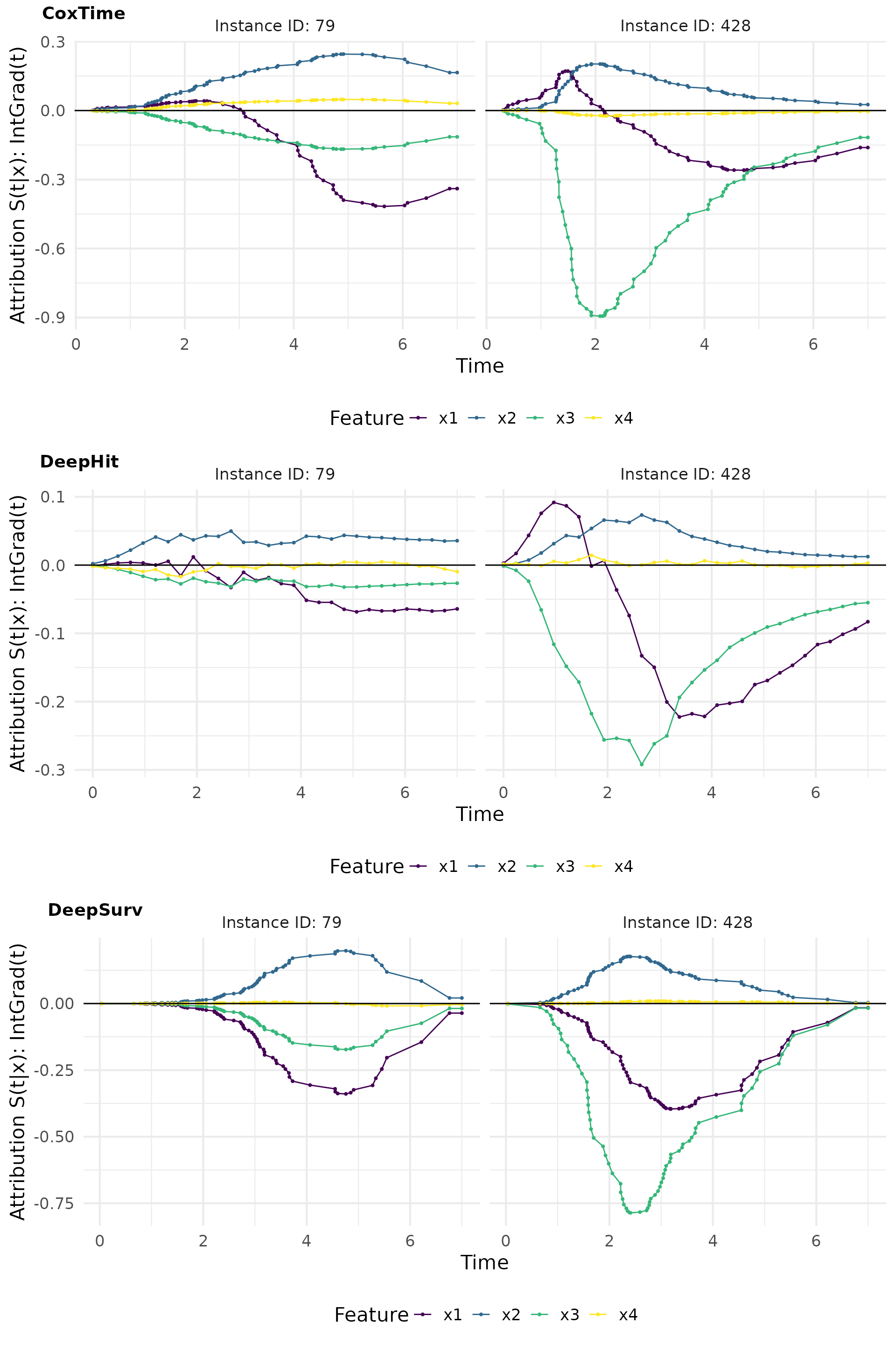

# Plot attributions
intgrad0_plot_comp <- cowplot::plot_grid(
  plot(ig0_cox, add_comp = "all", type = "attr"), 
  plot(ig0_deephit, add_comp = "all", type = "attr"), 
  plot(ig0_deepsurv, add_comp = "all", type = "attr"),
  nrow = 3, labels = c("CoxTime", "DeepHit", "DeepSurv"))
intgrad0_plot_comp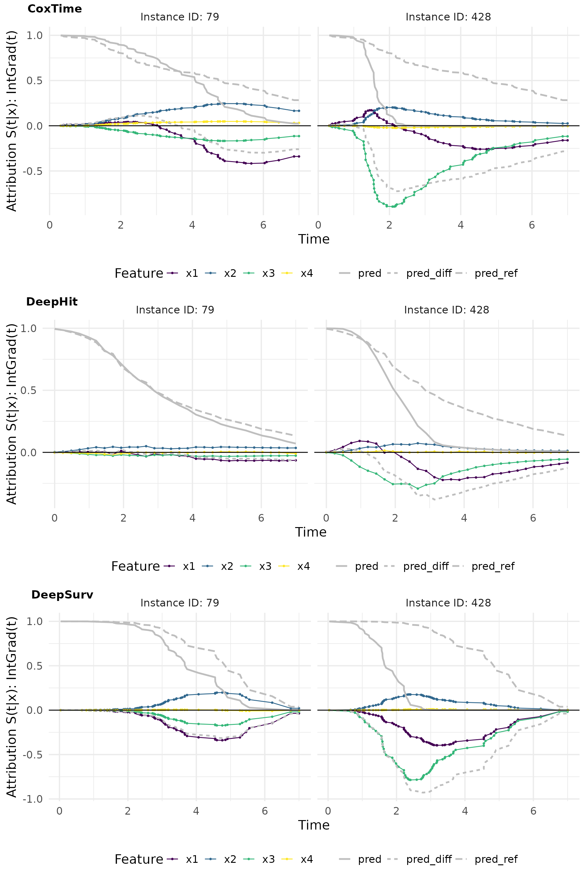

Contribution plots effectively visualize the normalized absolute contribution of each feature to the difference between reference and (survival) prediction over time.

# Plot contributions
intgrad0_plot_contr <- cowplot::plot_grid(
  plot(ig0_cox, type = "contr"), 
  plot(ig0_deephit, type = "contr"), 
  plot(ig0_deepsurv, type = "contr"),
  nrow = 3, labels = c("CoxTime", "DeepHit", "DeepSurv"))
intgrad0_plot_contr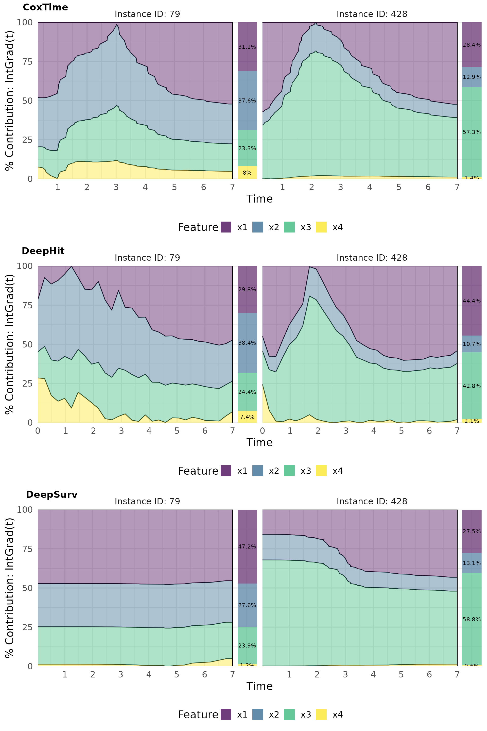

Complementarily, force plots emphasize the relative contribution and direction of each feature at a set of representative survival times.

# Plot force
intgrad0_plot_force <- cowplot::plot_grid(
  plot(ig0_cox, type = "force"),
  plot(ig0_deephit, type = "force"),
  plot(ig0_deepsurv, type = "force"),
  nrow = 3, labels = c("CoxTime", "DeepHit", "DeepSurv"))
intgrad0_plot_force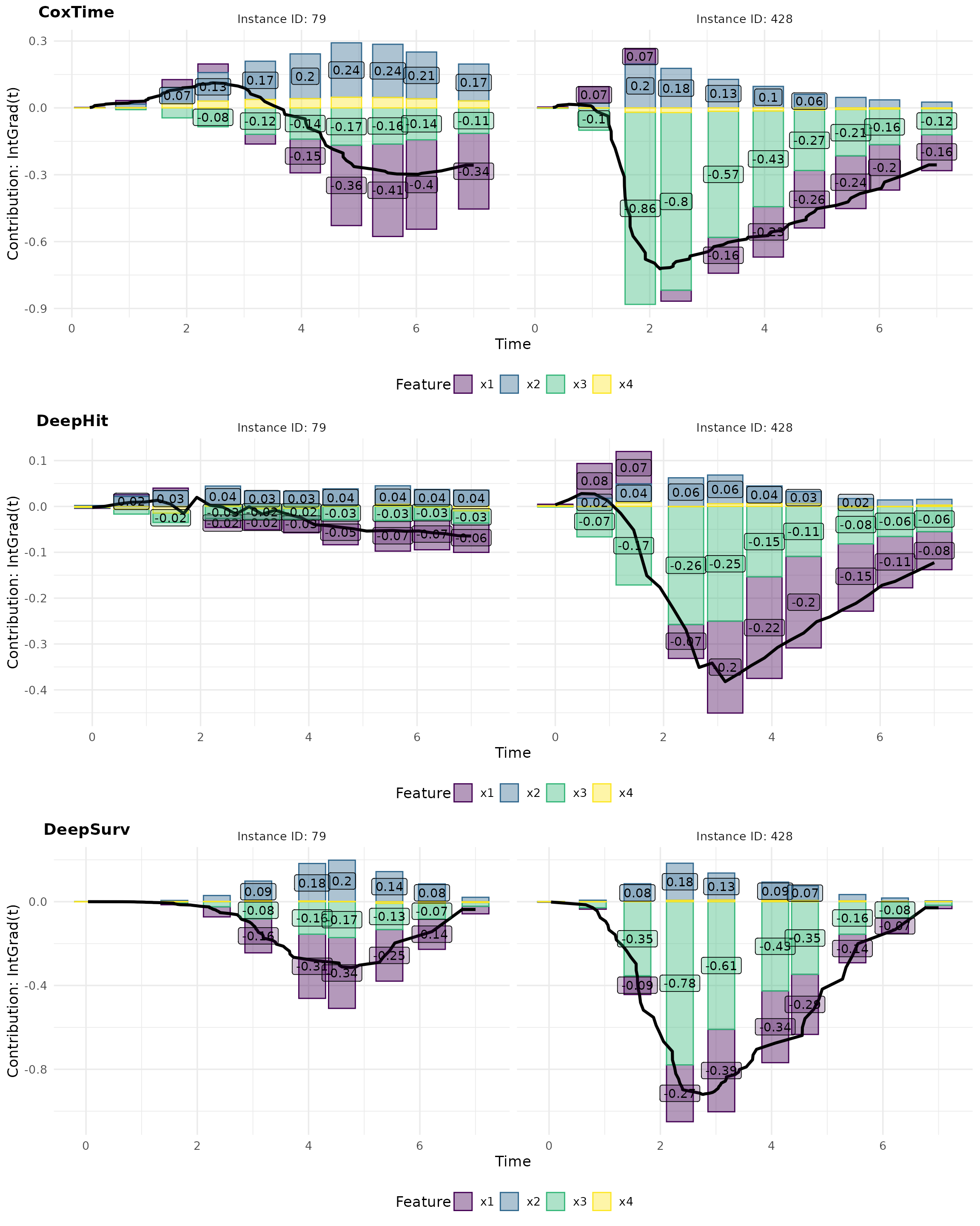

GradSHAP(t)

GradSHAP(t) is a method that computes the SHAP values for survival predictions. It provides a measure of the contribution of each feature to the survival predictions, taking into account the time-dependent effects.

# Compute GradShap(t)
gshap_cox <- surv_gradSHAP(exp_coxtime, instance = td_ids, n = 50, num_samples = 100)
gshap_deephit <- surv_gradSHAP(exp_deephit, instance = td_ids, n = 50, num_samples = 100)
gshap_deepsurv <- surv_gradSHAP(exp_deepsurv, instance = td_ids, n = 50, num_samples = 100)

# Plot attributions
gshap_plot <- cowplot::plot_grid(
  plot(gshap_cox, type = "attr"), 
  plot(gshap_deephit, type = "attr"), 
  plot(gshap_deepsurv, type = "attr"),
  nrow = 3, labels = c("CoxTime", "DeepHit", "DeepSurv"))
gshap_plot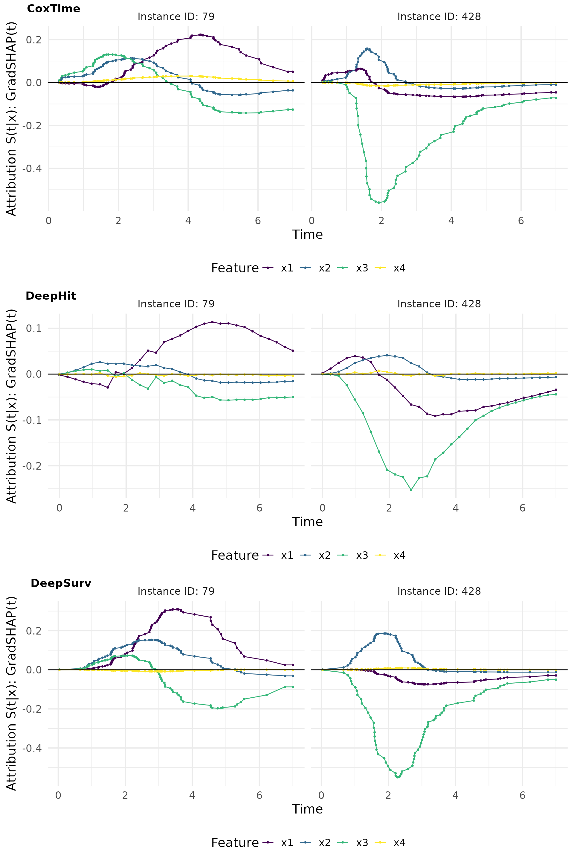

# Plot attributions
gshap_plot_comp <- cowplot::plot_grid(
  plot(gshap_cox, add_comp = "all", type = "attr"), 
  plot(gshap_deephit, add_comp = "all", type = "attr"), 
  plot(gshap_deepsurv, add_comp = "all", type = "attr"),
  nrow = 3, labels = c("CoxTime", "DeepHit", "DeepSurv"))
gshap_plot_comp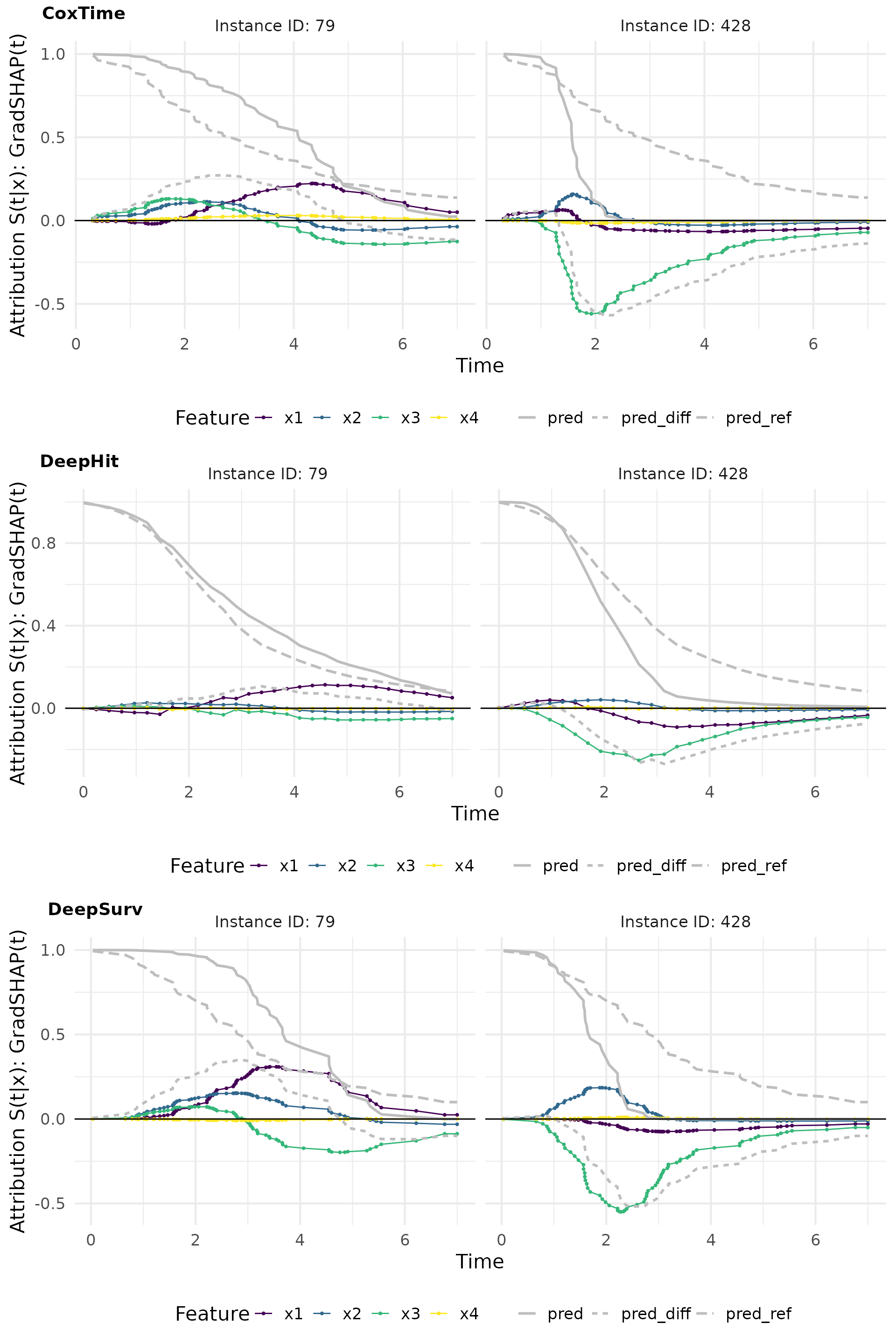

# Plot contributions
gshap_plot_contr <- cowplot::plot_grid(
  plot(gshap_cox, type = "contr"), 
  plot(gshap_deephit, type = "contr"), 
  plot(gshap_deepsurv, type = "contr"), 
  nrow = 3, labels = c("CoxTime", "DeepHit", "DeepSurv"))
gshap_plot_contr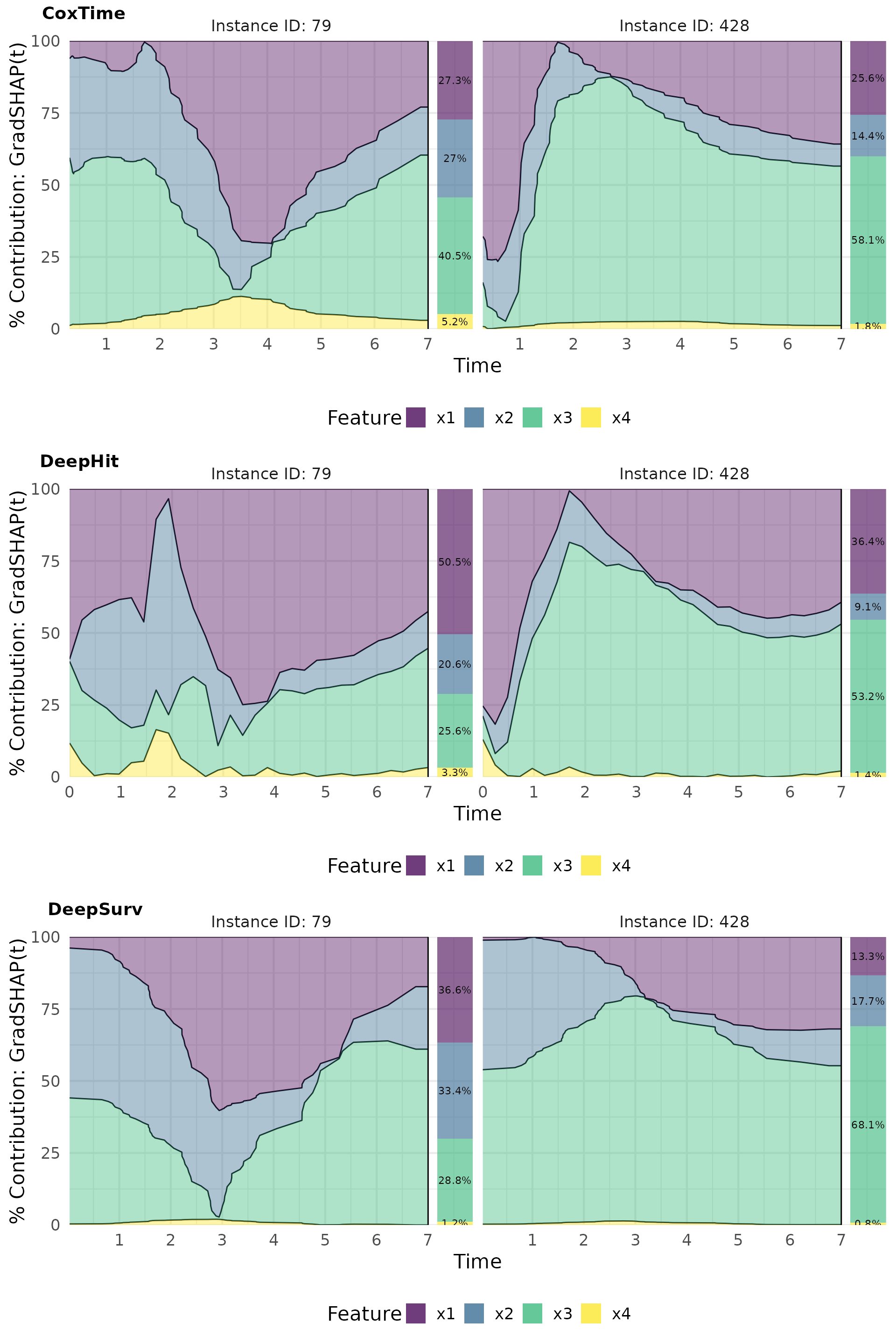

# Plot force
gshap_plot_force <- cowplot::plot_grid(
  plot(gshap_cox, type = "force"),
  plot(gshap_deephit, type = "force"),
  plot(gshap_deepsurv, type = "force"),
  nrow = 3, labels = c("CoxTime", "DeepHit", "DeepSurv"))
gshap_plot_force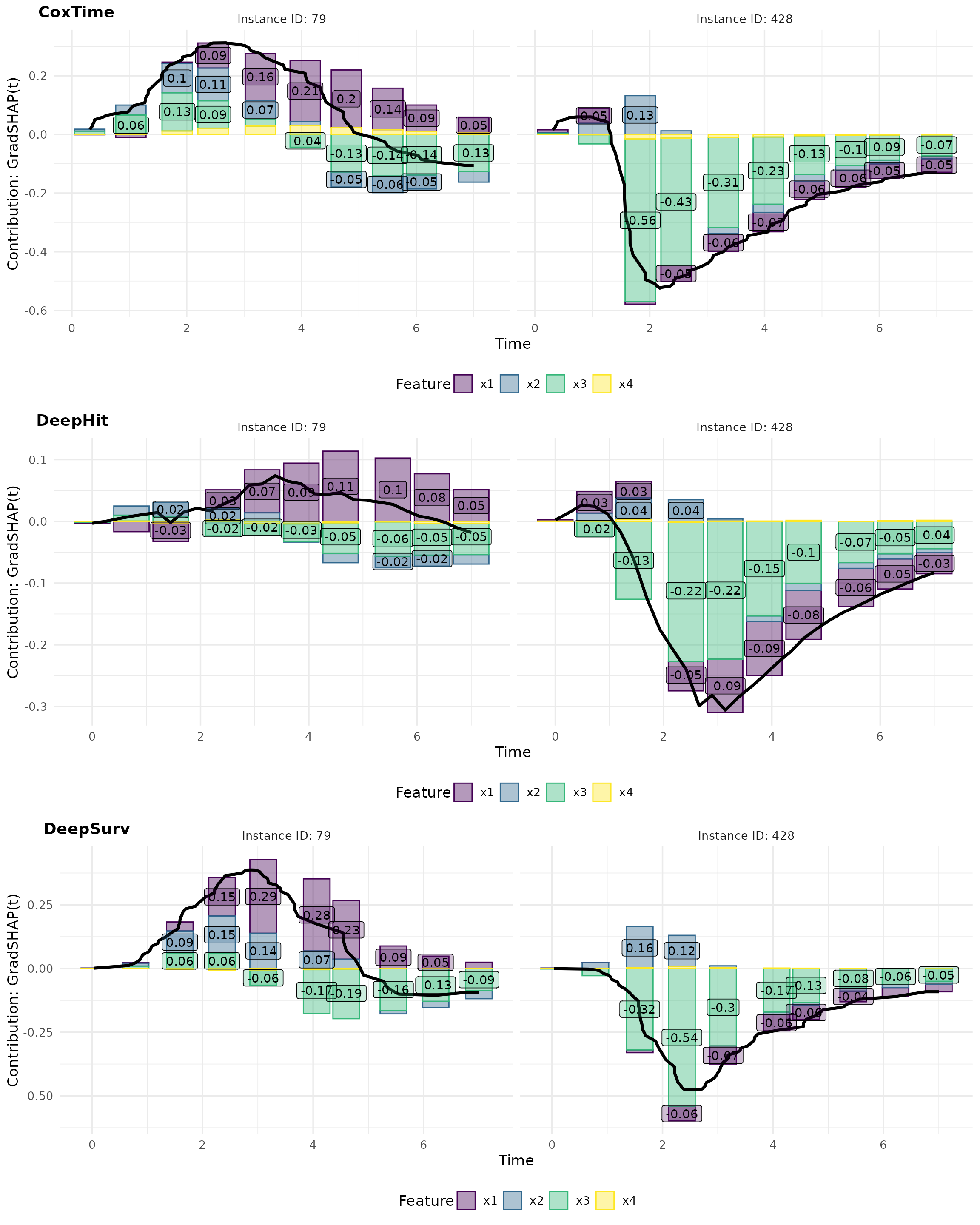

For example, the opposite effects of low vs. high values of $x_1$ are effectively captured in the plots. In observation 79, a low $x_1$ positively influences survival at later time points ( $t>2$ ) compared to the overall average survival in the dataset, resulting in its largest contributions occurring at these times. Conversely, in observation 428, a high $x_1$ induces substantial contributions at earlier time points ( $t<2$ ), but negatively impacts survival at later times, reflecting its early event as a consequence of the high $x_1$ and the strong negative effect of $x_3$ . The average normalized absolute contribution, displayed on the right side of the contribution plots, offers a time-independent measure of feature importance, confirming the dominance of $x_3$ for the survival prediction of instance 428. Additionally, the visualizations suggest that CoxTime partially attributes the time-varying effect of $x_1$ to the other features, as the model, being non-parametric and lacking explicit knowledge of the time-dependent functional form, struggles to precisely disentangle and localize this effect.