How to load my model?

library(survinng)
library(here)

The survinng package is designed in a flexible way to allow users to load models trained in R or Python using survivalmodels or pycox, respectively. Under the hood, the package uses the torch package and any base neural network can be loaded and will be coverted to the corresponding survival model, e.g., a DeepHit, DeepSurv, or CoxTime survival model.

Load a base `torch` model

This is the simplest way to load a model. The model must be a torch::nn_module and any input (tabular, image, multimodal, etc.) can be passed as long as the output dimension fits the expected survival deep learning architecture. This means:

For a DeepHit model, the output dimension must be of shape (batch_size, n_risks, n_time_bins) where n_risks is the number of competing risks and n_time_bins the number of time bins.
For a DeepSurv and CoxTime models, the output dimension must be of shape (batch_size, 1), since both models are designed to predict the risk of a single event and are Cox-based.

Example DeepHit model

In this example, we will create a simple DeepHit model using the torch package. The model will have 5 competing risks and 20 time bins. The input dimension will be 10 features. The model will be a simple feedforward neural network with two hidden layers. Important to note is that the output dimension is reshaped to (batch_size, n_risks, n_time_bins).

library(torch)

n_risks <- 5
n_time_bins <- 20
n_features <- 10

# Create the base model and data
base_model_deephit <- nn_module(
  initialize = function() {
    self$net <- nn_sequential(
      nn_linear(n_features, 128),
      nn_relu(),
      nn_linear(128, n_risks * n_time_bins)
    )
  },
  forward = function(x) {
    self$net(x) %>%
      torch_reshape(c(-1, n_risks, n_time_bins))
  }
)
model_deephit <- base_model_deephit()
data <- torch_randn(50, n_features)
time_bins <- seq(0, 10, length.out = n_time_bins)

# Check output
output <- model_deephit(data)
print(output$shape)
#> [1] 50  5 20

Now, we have our (untrained) base model and corresponding data. The next step is to create a survinng explainer object. This is done using the explain() function. The function takes the model, data, and time bins (required for a DeepHit model) as input and internally combines the base model with the DeepHit architecture. The model_type argument is set to "deephit" to indicate that the model is a DeepHit model. The function will return an explainer object which can be used to compute all implemented gradient-based feature attribution methods in the survival context.

# Create explainer object
exp_deephit <- survinng::explain(model_deephit, data = data, model_type = "deephit",
                                 time_bins = time_bins)
print(exp_deephit)
#> Explainer for DeepHit model
#> -----------------------------------
#> Model Class: DeepHit
#> Number of instances in the input data:  50 
#> Competing risks: Not specified
#> Number of time bins in the model:  20 
#> Model parameters:
#>  - Number of input modalities:  1 
#>  - Number of features:  10 
#>  - Preprocessing function applied: Yes
#> 
#> Features (first 5 shown):
#> X1, X2, X3, X4, X5 
#> -----------------------------------
#> To see more details, explore the individual elements of the object.

# Calculate gradients
grad <- surv_grad(exp_deephit, instance = c(1,3))

# Plot gradients
plot(grad)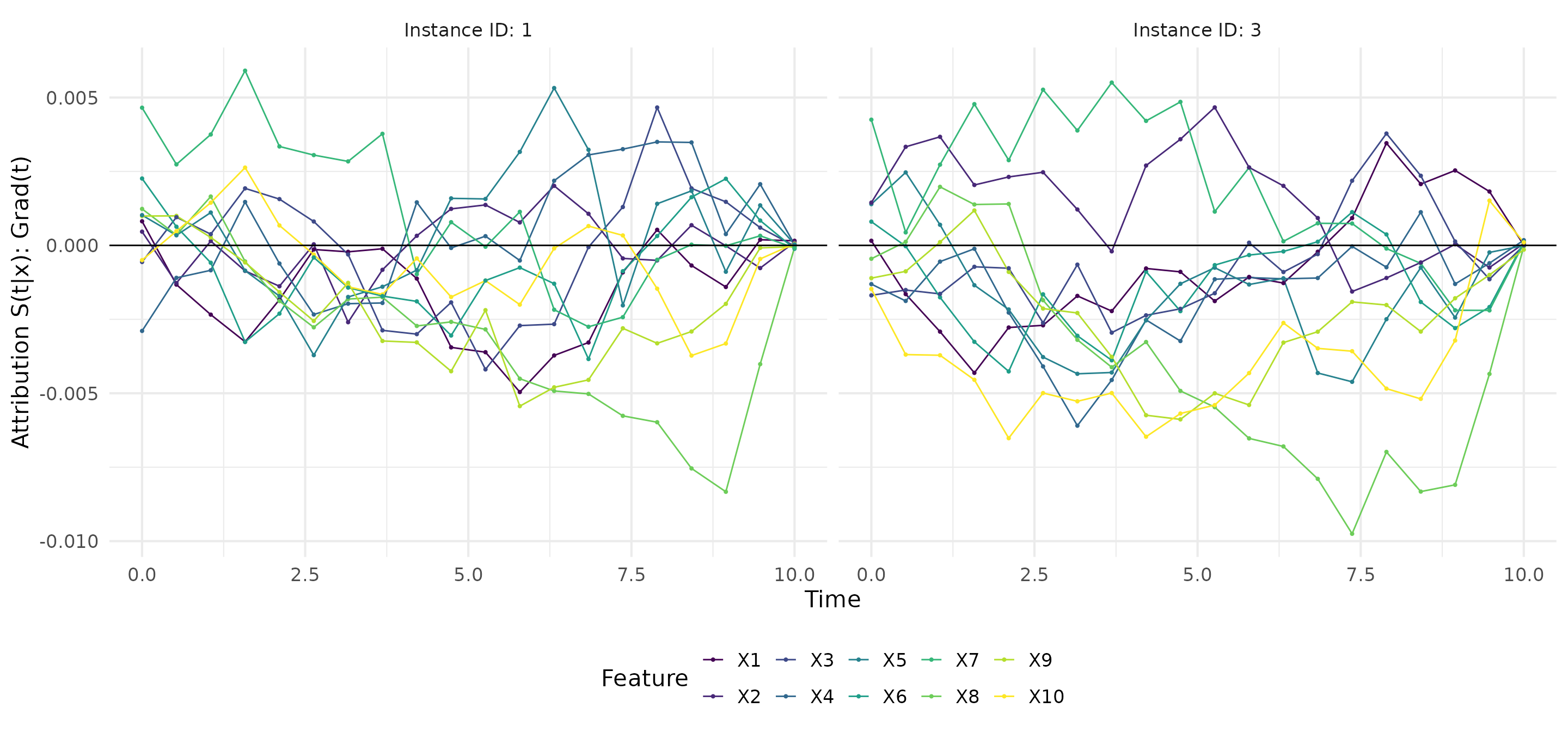

Example DeepSurv model

In this example, we will create a simple DeepSurv model using the torch package. Since DeepSurv is a Cox-based model, the output dimension will be of shape (batch_size, 1) and we need the baseline hazard function.

library(torch)

n_features <- 10

# Create baseline hazard function (50 time points)
time <- seq(0, 10, length.out = 50)
hazard <- exp(-(time - 5)^2 / 5)
base_hazard <- data.frame(time = time, hazard = hazard)

# Create the base model and data
base_model_deepsurv <- nn_module(
  initialize = function() {
    self$net <- nn_sequential(
      nn_linear(n_features, 128),
      nn_relu(),
      nn_linear(128, 1, bias = FALSE)
    )
  },
  forward = function(x) {
    self$net(x)
  }
)
model_deepsurv <- base_model_deepsurv()
data <- torch_randn(50, n_features)

# Check output
output <- model_deepsurv(data)
print(output$shape)
#> [1] 50  1

Now, we have our (untrained) base model and corresponding data, including the baseline hazard values The next step is to create a survinng explainer object. This is done using the explain() function. The function takes the model, data, and baseline hazard (required for a DeepSurv model) as input and internally combines the base model with the DeepSurv architecture. The model_type argument is set to "deepsurv" to indicate that the model is a DeepSurv model.

# Create explainer object
exp_deepsurv <- survinng::explain(model_deepsurv, data = data, 
                                  model_type = "deepsurv",
                                  baseline_hazard = base_hazard)
print(exp_deepsurv)
#> Explainer for DeepSurv model
#> -----------------------------------
#> Model Class: DeepSurv
#> Number of instances in the input data:  50 
#> Number of timepoints in the model:  50 (min: 0 , max: 10 )
#> Model parameters:
#>  - Number of input modalities:  1 
#>  - Number of features:  10 
#>  - Baseline hazard function: Yes
#>  - Preprocessing function applied: Yes
#> 
#> Features (first 5 shown):
#> X1, X2, X3, X4, X5 
#> -----------------------------------
#> To see more details, explore the individual elements of the object.

# Calculate IntGrad(t)
ig <- surv_intgrad(exp_deepsurv, instance = c(1,3))

# Show results as a contribution plot
plot(ig, type = "contr")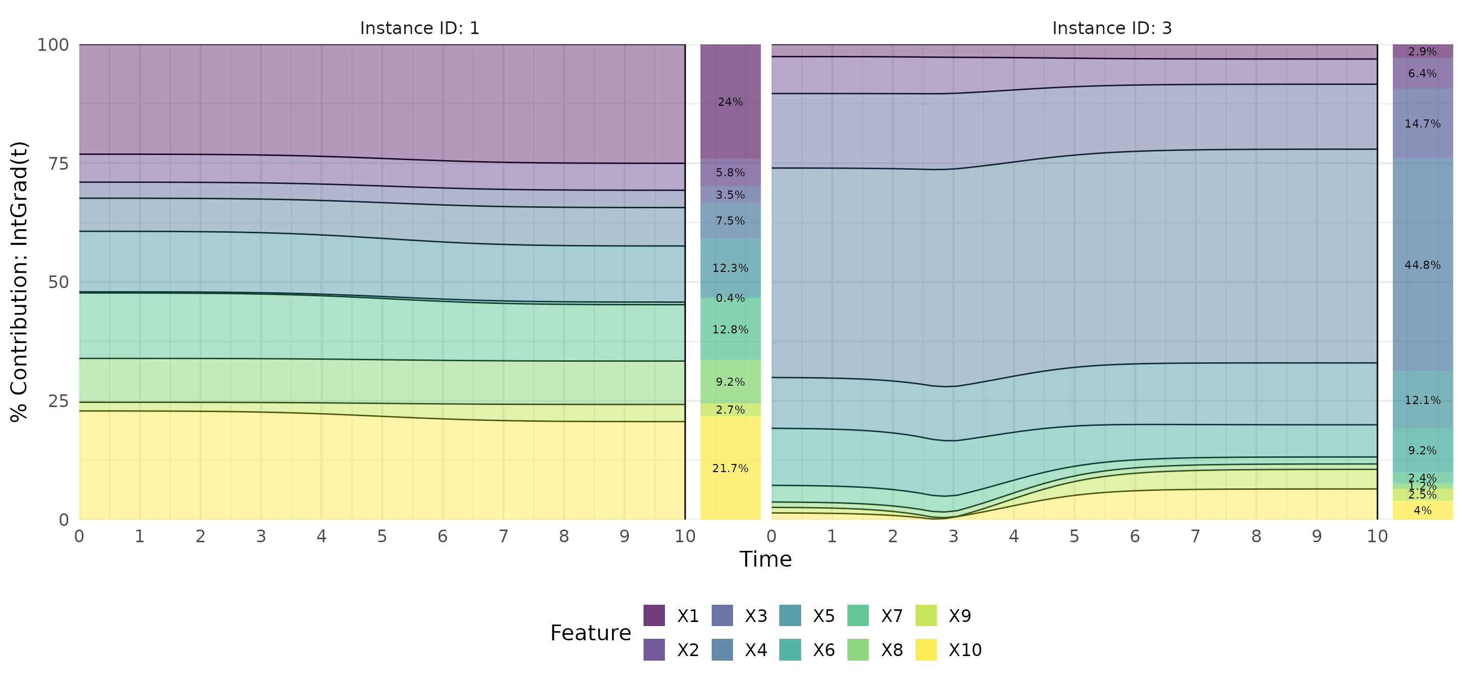

Example CoxTime model

In this example, we will create a simple CoxTime model using the torch package. It is very similar to the DeepSurv modelm i.e., the output dimension of the base model will be of shape (batch_size, 1) and we need the baseline hazard function since it is a Cox-based model. However, the time points are integrated to the input features, so the model will have n_features + 1 input features. Currently, the default function for adding the time points to the input features is the following one and assumes tabular data:

n_features <- 10
x <- torch_randn(50, n_features)
t <- torch_linspace(0, 10, steps = 50)

preprocess_fun <- function(x) {
  batch_size <- x$size(1)
  
  # Input (batch_size, n_features) -> (batch_size * t, n_features) (replicate each row t times)
  res <- x$repeat_interleave(length(t), dim = 1)
  
  # Add time to input
  time <- torch_vstack(replicate(batch_size, t$unsqueeze(-1)))
  
  # Combine both and return
  torch::torch_cat(list(res, time), dim = -1)
}

# Input shape
print(x$shape)
#> [1] 50 10

# Shape after preprocessing
preprocess_fun(x)$shape
#> [1] 2500   11

However, you can pass your own preprocessing function to the explain() function using the preprocess_fun argument, but this option is still experimental and not fully tested.

In the following code, we create the base model and data for the CoxTime architecture. The model will have 10 + 1 features and 50 time points for the baseline hazard function (this is basically the same as the DeepSurv model from this Section):

library(torch)
n_features <- 10

# Create baseline hazard function (50 time points)
time <- seq(0, 10, length.out = 50)
hazard <- exp(-(time - 5)^2 / 5)
base_hazard <- data.frame(time = time, hazard = hazard)

# Create the base model and data
base_model_coxtime <- nn_module(
  initialize = function() {
    self$net <- nn_sequential(
      nn_linear(n_features + 1, 128),
      nn_relu(),
      nn_linear(128, 1, bias = FALSE)
    )
  },
  forward = function(x) {
    self$net(x)
  }
)
model_coxtime <- base_model_coxtime()
data <- torch_randn(50, n_features)

# Check output
output <- model_coxtime(preprocess_fun(data))
print(output$shape) # the instances are replicated t times
#> [1] 2500    1

Now, we have our (untrained) base model and corresponding data, including the baseline hazard values. The next step is to create a survinng explainer object. This is done using the explain() function. The function takes the model, data, and baseline hazard (required for a CoxTime model) as input and internally combines the base model with the CoxTime architecture. The model_type argument is set to "coxtime" to indicate that the model is a CoxTime model. The preprocess_fun argument is set to the function we defined earlier to add the time points to the input features.

# Create explainer object
exp_coxtime <- survinng::explain(model_coxtime, data = data, 
                                 model_type = "coxtime",
                                 baseline_hazard = base_hazard)
print(exp_coxtime)
#> Explainer for CoxTime model
#> -----------------------------------
#> Model Class: CoxTime
#> Number of instances in the input data:  50 
#> Number of timepoints in the model:  50 
#> Model parameters:
#>  - Number of input modalities:  1 
#>  - Number of features:  10 
#>  - Baseline hazard function: Yes
#>  - Preprocessing function applied: Yes
#> 
#> Features (first 5 shown):
#> X1, X2, X3, X4, X5 
#> -----------------------------------
#> To see more details, explore the individual elements of the object.

# Calculate IntGrad(t)
ig <- surv_intgrad(exp_coxtime, instance = c(1,3))

# Show results as a contribution plot
plot(ig, type = "contr")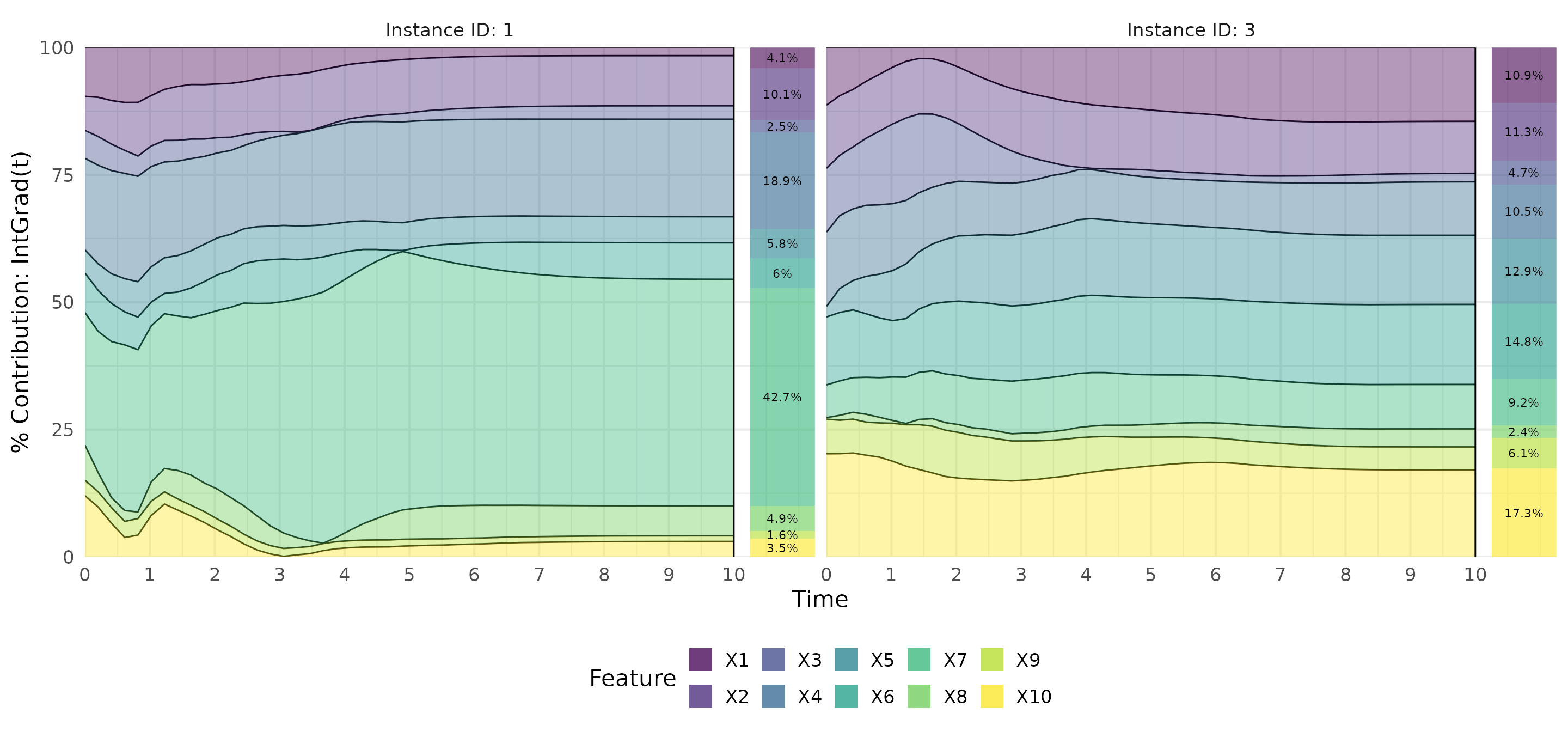

Load a `survivalmodels` model

The survivalmodels package is a R package for survival analysis using deep learning. Especially for the deep learning models, it uses the pycox package in Python under the hood via reticulate. The survinng package is designed to load models trained in survivalmodels directly. However, there are some issues when torch in R (i.e., LibTorch) and Pytorch in Python are loaded in the same session (see issue #815). Therefore, we keep the training procedure using survivalmodels in a separate session using callr.

In the following example, we will train a default DeepHit, DeepSurv and Coxtime model using the survivalmodels package. The models will be trained on the lung dataset from the survival package.

library(survival)
library(callr)

# Load lung dataset
data(cancer, package = "survival")
data <- na.omit(cancer[, c(1, 4, 5, 6, 7, 10, 2, 3)])

# Train models in separate session
models <- callr::r(function(data) {
  library(survivalmodels)
  library(survival)
  
  # Set seed for reproducibility
  set.seed(42)
  set_seed(42)
  
  # Make sure pycox is installed
  install_pycox(install_torch = TRUE)
  
  # Fit the DeepSurv model
  fit_deepsurv <- deepsurv(Surv(time, status) ~ ., data = data, epochs = 10,
                           num_nodes = 8L)
  
  # Fit the DeepHit model
  fit_deephit <- deephit(Surv(time, status) ~ ., data = data, epochs = 10,
                         cuts = 30, num_nodes = 8L)
  
  # Fit the CoxTime model
  fit_coxtime <- coxtime(Surv(time, status) ~ ., data = data, epochs = 10,
                         num_nodes = 8L)

  # Extract the models using `survinng`
  ext_deepsurv <- survinng::extract_model(fit_deepsurv)
  ext_deephit <- survinng::extract_model(fit_deephit)
  ext_coxtime <- survinng::extract_model(fit_coxtime)
  
  # Return the extracted models
  list(deepsurv = ext_deepsurv, deephit = ext_deephit, coxtime = ext_coxtime)
}, args = list(data = data))

Now, we have our trained models in the models list. The models are extracted using the extract_model() function from the survinng package. These objects and the data to be explained can be passed to the explain() function to create the survinng explainer objects.

# Create explainer objects
exp_deepsurv <- survinng::explain(models$deepsurv, data = data)
exp_deephit <- survinng::explain(models$deephit, data = data)
exp_coxtime <- survinng::explain(models$coxtime, data = data)

The explain() function will automatically detect the model type and create the corresponding explainer object, i.e., the model_type argument is not needed in this case. Using the explainer objects, we can compute the gradient-based feature attribution methods. The instance argument is used to specify the instances for which the explanations should be computed.

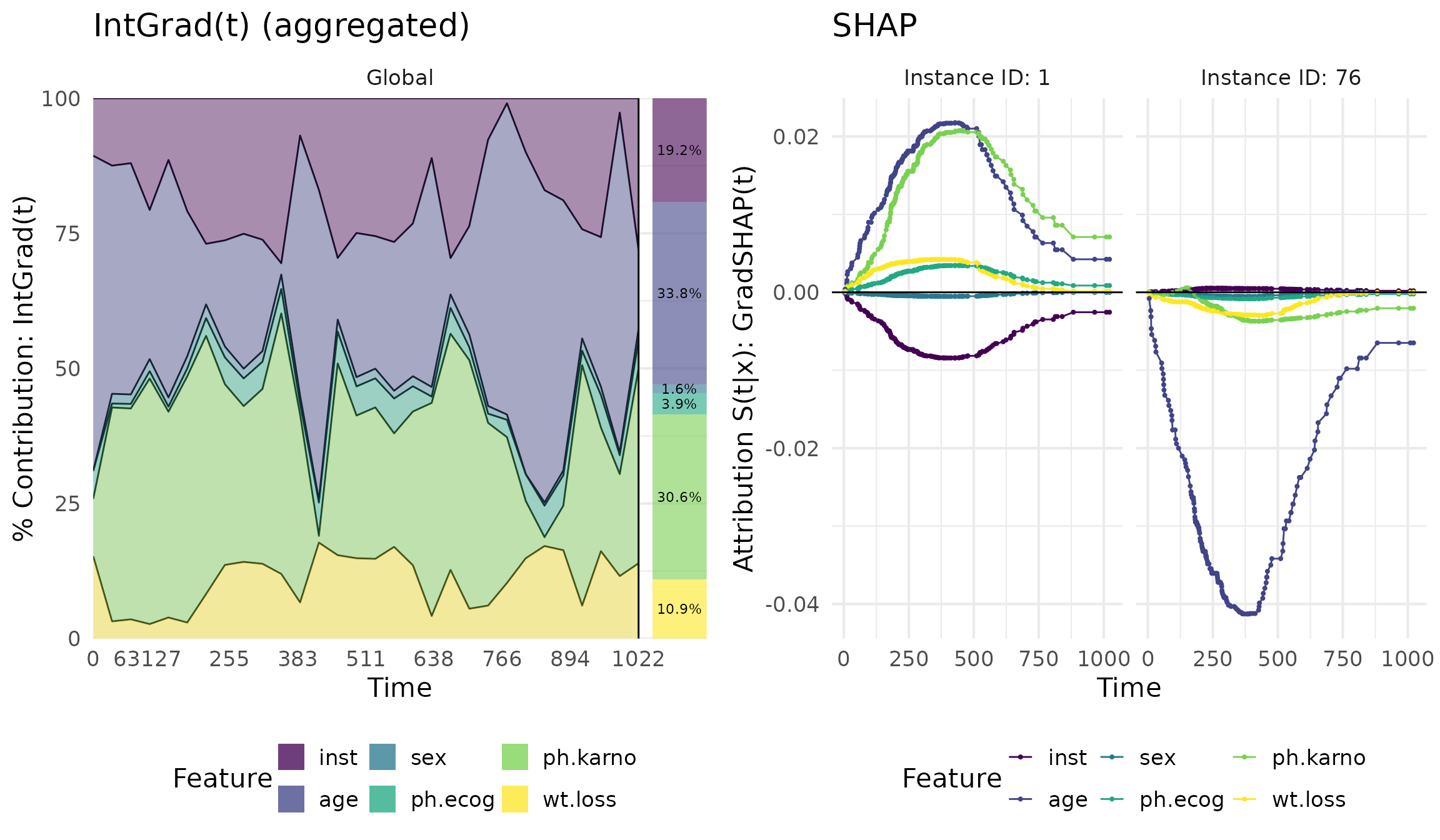
# Show instances to be explained
ids <- c(1, 76)
data[ids, ]
#>    inst age sex ph.ecog ph.karno wt.loss time status
#> 2     3  68   1       0       90      15  455      2
#> 83   11  42   1       1       80       8  196      1

# Calculate feature attribution methods
grad <- surv_grad(exp_deepsurv, instance = ids)
ig <- surv_intgrad(exp_deephit, instance = ids)
shap <- surv_gradSHAP(exp_coxtime, instance = ids)

# Show the predictions
plot(shap, type = "pred")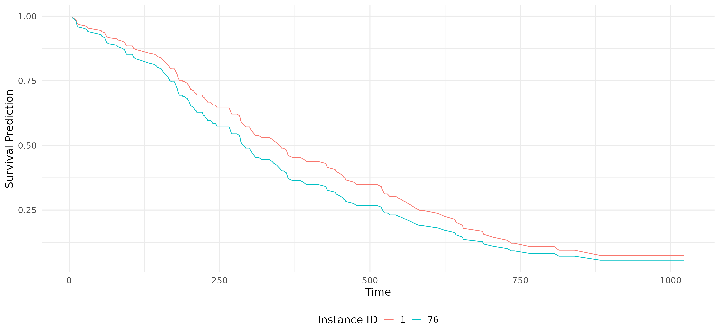

With the plot() function, we can visualize the results. The type argument can be set to "pred" to show the predictions of the model, "attr" to show the feature attribution values, or "contr" to show the contribution plots.

library(cowplot)
library(ggplot2)

plot_grid(
  plot(ig, type = "contr", aggregate = TRUE) + ggtitle("IntGrad(t) (aggregated)"),
  plot(shap, type = "attr") + ggtitle("SHAP"),
  ncol = 2
)

Load a `pycox` Python model

It is also possible to load models trained in Python using the pycox package. Basically, it is the same procedure as for another torch::nn_module model. The only difference is that the model needs to be loaded in R as described in the Pyton to R article for the torch package. This means, the model architecture must be rebuilt in R and the weights and parameters must be loaded from the Python model.

For illustration, we will use the same CoxTime model from the pycox Jupyter notebook here on the METABRIC dataset. After training the model, follow these steps to extract the base hazard function and the model weights (model and x_test are defined as in the mentioned notebook):

import pandas as pd

# We use only a sample of the data for the baseline hazard
base_hazard = model.compute_baseline_hazards(sample = 200)

# Save base hazard as csv
pd_base_hazard = pd.DataFrame({
    'time': base_hazard.index.to_numpy(), 
    'hazard': base_hazard.to_numpy()})
pd_base_hazard.to_csv('base_hazard.csv', index = False)

# Save model weights (not the  whole model!)
torch.save(model.net.net.state_dict(), 'model.pt')

# Save data to be explained
df_train.to_csv('df_train.csv', index=False)
pd.DataFrame(x_val, columns = df_val.columns[0:9]).to_csv('x_val.csv', index=False)

Now, the tricky part is rebuilding the model architecture in R with the same names and parameters as in the Python model. This is done in the following code:

# Rebuild a dense layer
BaseMLP_dense <- nn_module(
  initialize = function(in_feat, out_feat) {
    self$linear <- nn_linear(in_feat, out_feat)
    self$batch_norm <- nn_batch_norm1d(out_feat)
  },

  forward = function(x) {
    x <- self$linear(x)
    x <- nn_relu()(x)
    x <- self$batch_norm(x)
  }
)

# Rebuild the whole model
BaseMLP <- torch::nn_module(
  classname = "BaseMLP",
  initialize = function() {
    
    self$net <- nn_sequential(
      BaseMLP_dense(10, 32),
      BaseMLP_dense(32, 32),
      nn_linear(32, 1, bias = FALSE)
    )
  },
  forward = function(x) {
    if (is.list(x)) x <- x[[1]]
    self$net(x)
  }
)

# Create model and load state dict
model <- BaseMLP()
state_dict <- load_state_dict(here("vignettes/articles/how_to_load_model/model.pt"))
model$load_state_dict(state_dict)
model$eval()
print(model)
#> An `nn_module` containing 1,568 parameters.
#> 
#> ── Modules ─────────────────────────────────────────────────────────────────────
#> • net: <nn_sequential> #1,568 parameters

The model architecture is now rebuilt in R and the weights are loaded from the Python model. The next step is to load the baseline hazard function and the data to be explained. Additionally, since in the notebook uses a label transformation, we need to rebuild the transformation function in R. However, this is a simple mean and standard deviation transformation, so we can use the labtrans argument in the explain() function to define the transformation function. The labtrans argument is a list with two functions: transform and transform_inv.

# Load base hazard and data
base_hazard <- read.csv(here("vignettes/articles/how_to_load_model/base_hazard.csv"))
df_train <- read.csv(here("vignettes/articles/how_to_load_model/df_train.csv"))
x_val <- read.csv(here("vignettes/articles/how_to_load_model/x_val.csv"))

# Rebuild the label transformation
mean <- mean(df_train$duration)
sd <- sd(df_train$duration)
labtrans <- list(
  transform = function(x) (x - mean) / sd,
  transform_inv = function(x) x * sd + mean
)

Now, we can create the survinng explainer object using the explain() function and apply all implemented gradient-based feature attribution methods on this model. The model_type argument is set to "coxtime" to indicate that the model is a CoxTime model and the labtrans argument is set to the defined transformation.

# Create explainer
explainer <- survinng::explain(model, data = x_val, model_type = "coxtime",
                               baseline_hazard = base_hazard,
                               labtrans = labtrans)

# Calculate GradSHAP(t)
grad_shap <- surv_gradSHAP(explainer, instance = c(1, 3))

# Show predictions
p1 <- plot(grad_shap, type = "pred")

# Show attribution results
p2 <- plot(grad_shap, type = "attr", add_comp = c("pred_diff"))

# Show contribution percentages
p3 <- plot(grad_shap, type = "contr")

cowplot::plot_grid(p1, p2, p3, ncol = 1)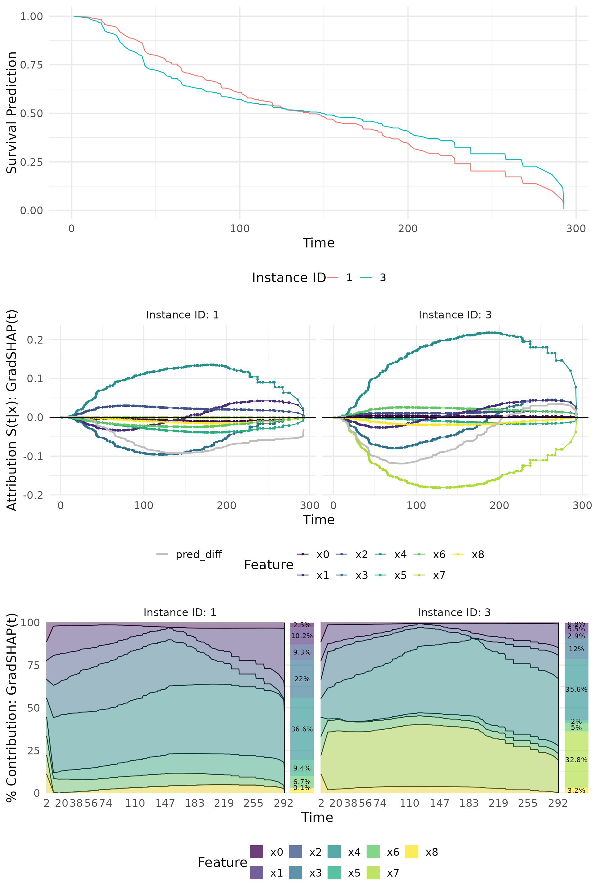

In a similar way, you can also load DeepSurv and DeepHit models from pycox. The only difference is that the model architecture must be changed accordingly. The model_type argument is set to "deepsurv" or "deephit" to indicate the model type.

Load a base torch model