Simulation of Time-independent Effects • survinng

In this vignette we simulate survival data to detect time-independent feature effects using gradient-based explanation techniques for survival neural network models.

Load the necessary libraries and source the utility functions.

library(survinng)
library(ggplot2)
library(cowplot)
library(dplyr)
library(tidyr)
library(survival)
library(survminer)
library(torch)
library(viridis)
library(here)

# Set seed for reproducibility
set.seed(2025)
torch_manual_seed(2025)

Preprocessing

Generate the data

We consider a simulated dataset with the following characteristics:

Sample size: 10,000 individuals
- 9,500 samples used for training
- 500 samples used for testing
Covariates:
- $X_1 \sim N(0, 1)$ : has a positive effect on the hazard
  → Negative effect on survival
- $X_2 \sim U(0, 1)$ : has a strong negative effect on the hazard
  → Positive effect on survival
- $X_3 \sim U(-1, 1)$ : has no effect on the hazard or survival
Time-dependency: None of the covariates have time-varying effects

Load Models and Data

The models used in this vignette are the same as those used in the main paper. The models were trained using the survivalmodels package, and the training process is not shown here, but can be found in the vignettes/articles/Sim_time_independent directory or on GitHub.

# Load data
train <- readRDS(here("vignettes/articles/Sim_time_independent/train.rds"))
test <- readRDS(here("vignettes/articles/Sim_time_independent/test.rds"))
dat <- rbind(train, test)

# Load extracted models
ext_coxtime <- readRDS(here("vignettes/articles/Sim_time_independent/ext_coxtime.rds"))
ext_deepsurv <- readRDS(here("vignettes/articles/Sim_time_independent/ext_deepsurv.rds"))
ext_deephit <- readRDS(here("vignettes/articles/Sim_time_independent/ext_deephit.rds"))

Performance

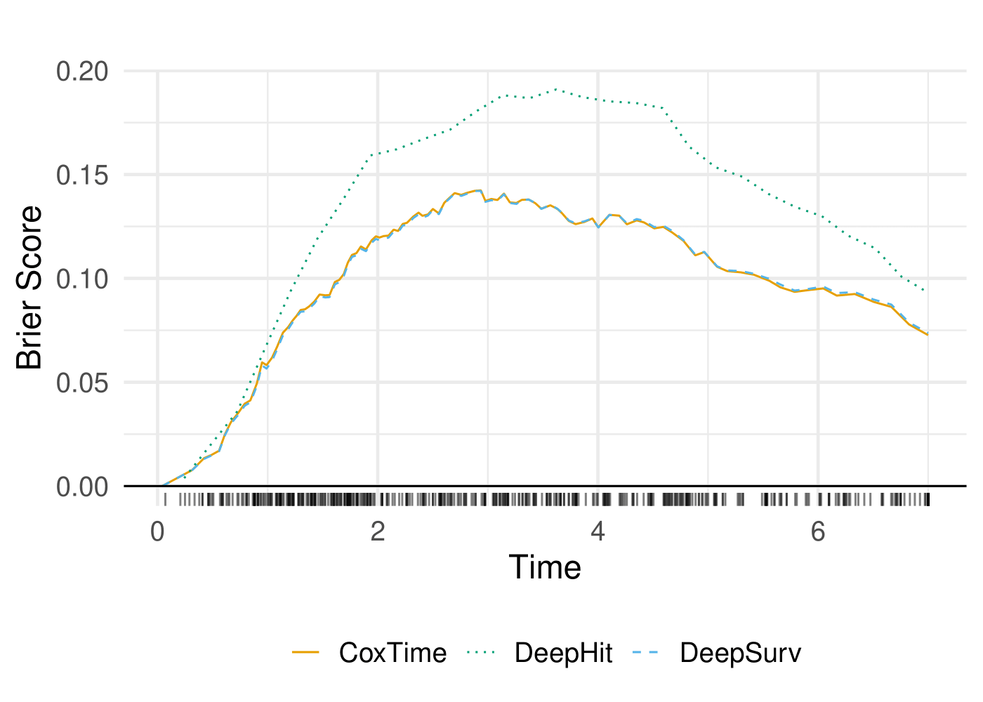
The performance of the models is evaluated using the C-Index and Integrated Brier Score (IBS). The C-Index measures the concordance between predicted and observed survival times, while the IBS quantifies the accuracy of survival predictions.

Model	C-Index	IBS
CoxTime	0.809372	0.099053
DeepSurv	0.809121	0.099031
DeepHit	0.808829	0.141614

Create Explainer

The explain() function creates an explainer object for the survival models. The data argument specifies the dataset used for explanation, and the model argument specifies the model to be explained. The target argument indicates the type of prediction to be explained (e.g., “survival”, “risk”, “cumulative hazard”).

exp_deephit <- survinng::explain(ext_deephit[[1]], data = test)
exp_coxtime <- survinng::explain(ext_coxtime[[1]], data = test)
exp_deepsurv <- survinng::explain(ext_deepsurv[[1]], data = test)

Survival Prediction

The survival predictions for the test dataset are computed using the predict() function. The type argument specifies the type of prediction to be made (e.g., “survival”, “risk”, “cumulative hazard”). The survival predictions are then plotted for a set of instances of interest.

# Print instances of interest
tid_ids <- c(13, 387)
print(test[tid_ids, ])
#>           time status        x1        x2          x3
#> 343  2.6653596      1 -0.434617 0.1162303 -0.08053765
#> 7906 0.9577924      1  2.454611 0.2462072 -0.04249294

# Compute Vanilla Gradient
grad_cox <- surv_grad(exp_coxtime, target = "survival", instance = tid_ids)
grad_deephit <- surv_grad(exp_deephit, target = "survival", instance = tid_ids)
grad_deepsurv <- surv_grad(exp_deepsurv, target = "survival", instance = tid_ids)

# Plot survival predictions
surv_plot <- cowplot::plot_grid(
  plot(grad_cox, type = "pred"),
  plot(grad_deephit, type = "pred"),
  plot(grad_deepsurv, type = "pred"),
  nrow = 1, labels = c("CoxTime", "DeepHit", "DeepSurv"),
  label_x = 0.03,      
  label_size = 14) 
surv_plot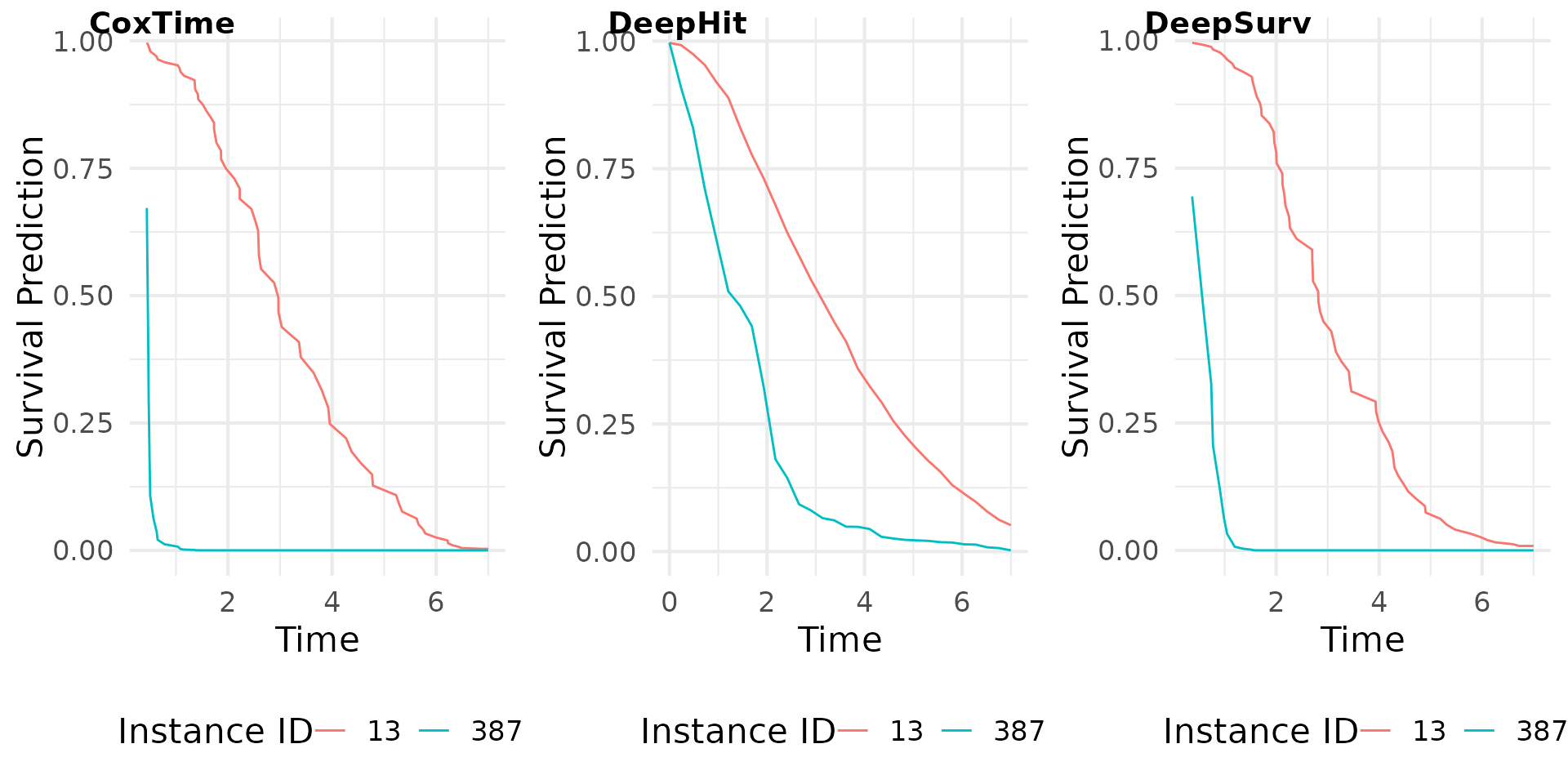

Explainable AI

The following sections demonstrate the application of various gradient-based explanation methods to the survival models. The methods include Grad(t), SmoothGrad(t), G x I(t), SmoothGrad x I(t), IntGrad(t), and GradSHAP(t). Each method provides insights into the contributions of the covariates to the survival predictions.

Grad(t) (Sensitivity)

Here we compute the gradient of the survival predictions with respect to the input features. The surv_grad() function computes the gradients for the specified instances.

# Plot attributions
grad_plot <- cowplot::plot_grid(
  plot(grad_cox, type = "attr"),
  plot(grad_deephit, type = "attr"),
  plot(grad_deepsurv, type = "attr"),
  nrow = 3, labels = c("CoxTime", "DeepHit", "DeepSurv"))
grad_plot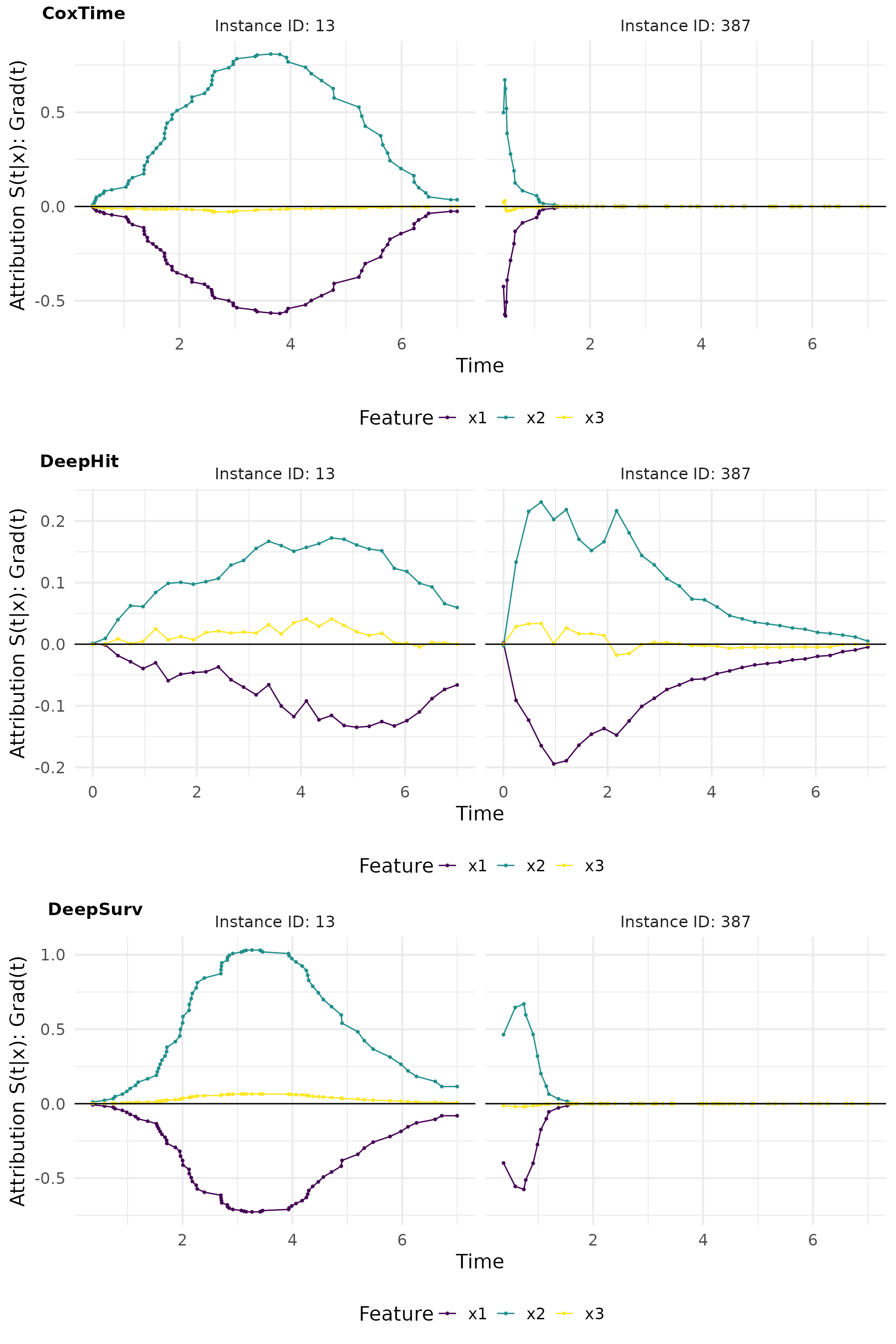

SmoothGrad(t) (Sensitivity)

SmoothGrad(t) is a method that adds noise to the input features and computes the average gradient over multiple noisy samples. This approach helps to reduce the noise in the gradient estimates and provides a clearer picture of the feature importance.

# Compute SmoothGrad
sg_cox <- surv_smoothgrad(exp_coxtime, target = "survival", instance = tid_ids, n = 50, noise_level = 0.1)
sg_deephit <- surv_smoothgrad(exp_deephit, target = "survival", instance = tid_ids, n = 50, noise_level = 0.1)
sg_deepsurv <- surv_smoothgrad(exp_deepsurv, target = "survival", instance = tid_ids, n = 50, noise_level = 0.1)

# Plot attributions
smoothgrad_plot <- cowplot::plot_grid(
  plot(sg_cox, type = "attr"), 
  plot(sg_deephit, type = "attr"), 
  plot(sg_deepsurv, type = "attr"),
  nrow = 3, labels = c("CoxTime", "DeepHit", "DeepSurv"))
smoothgrad_plot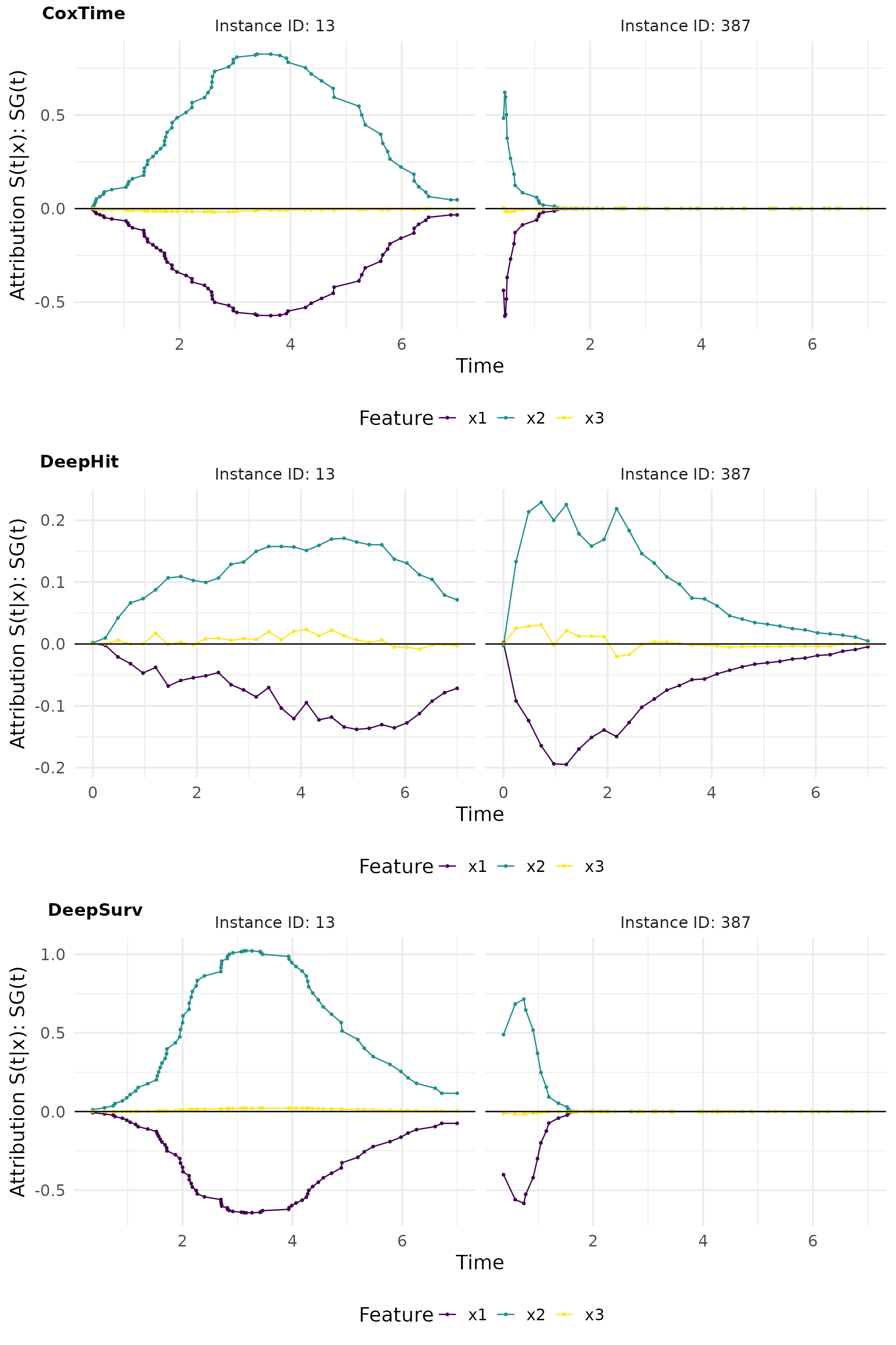

Grad x I(t)

Grad x I(t) is a method that computes the gradient of the survival predictions with respect to the input features and multiplies it by the survival predictions themselves. This approach provides insights into the true local effects of the covariates on the survival prediction.

# Compute GradientxInput
gradin_cox <- surv_grad(exp_coxtime, instance = tid_ids, times_input = TRUE)
gradin_deephit <- surv_grad(exp_deephit, instance = tid_ids, times_input = TRUE)
gradin_deepsurv <- surv_grad(exp_deepsurv, instance = tid_ids, times_input = TRUE)

# Plot attributions
gradin_plot <- cowplot::plot_grid(
  plot(gradin_cox, type = "attr"), 
  plot(gradin_deephit, type = "attr"), 
  plot(gradin_deepsurv, type = "attr"),
  nrow = 3, labels = c("CoxTime", "DeepHit", "DeepSurv"))
gradin_plot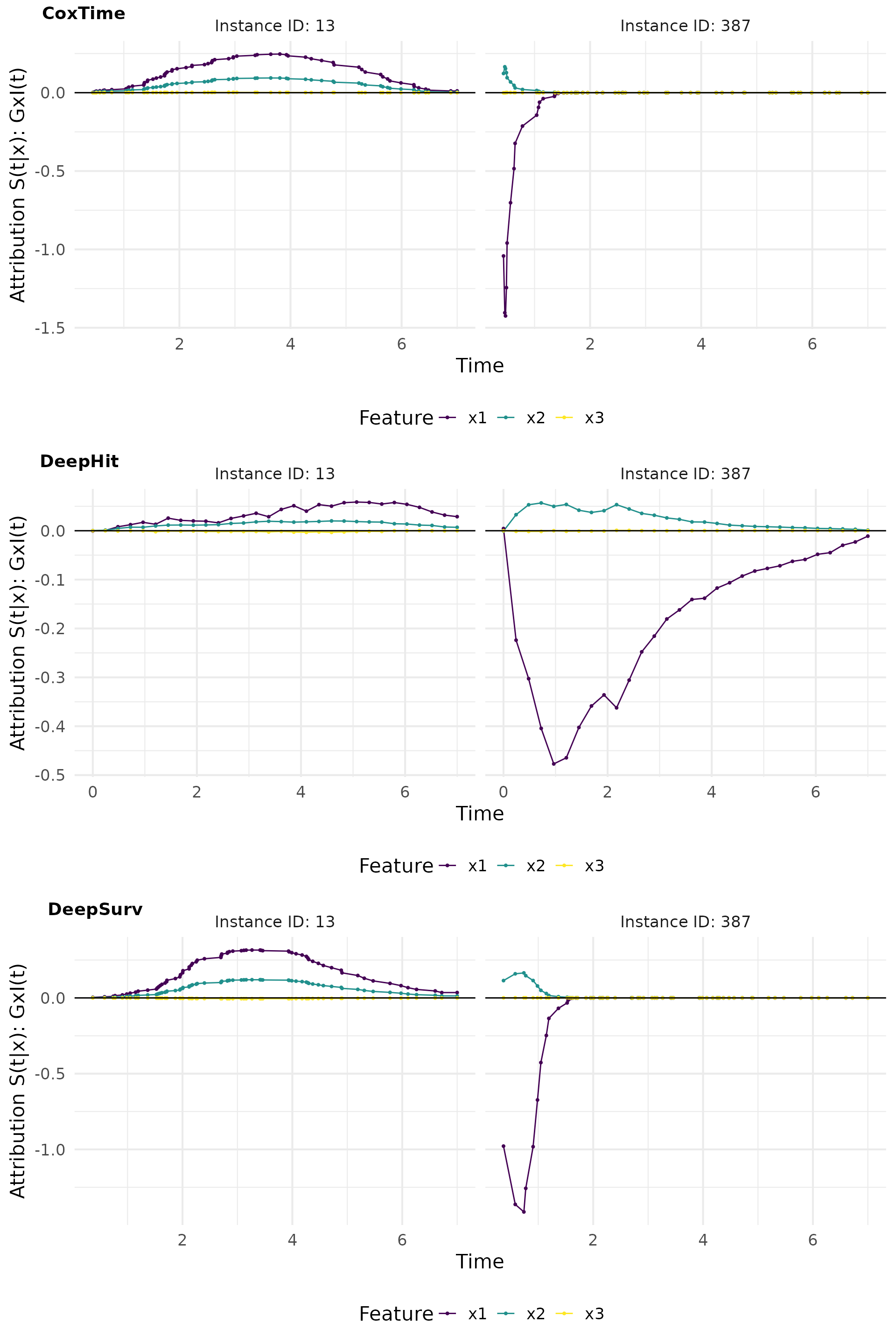

# Plot attributions
grad_gradin_plot <- cowplot::plot_grid(
  plot(grad_deepsurv, type = "attr") ,
  plot(gradin_deepsurv, type = "attr"),
  nrow = 2, labels = c("DeepSurv", "DeepSurv"))
grad_gradin_plot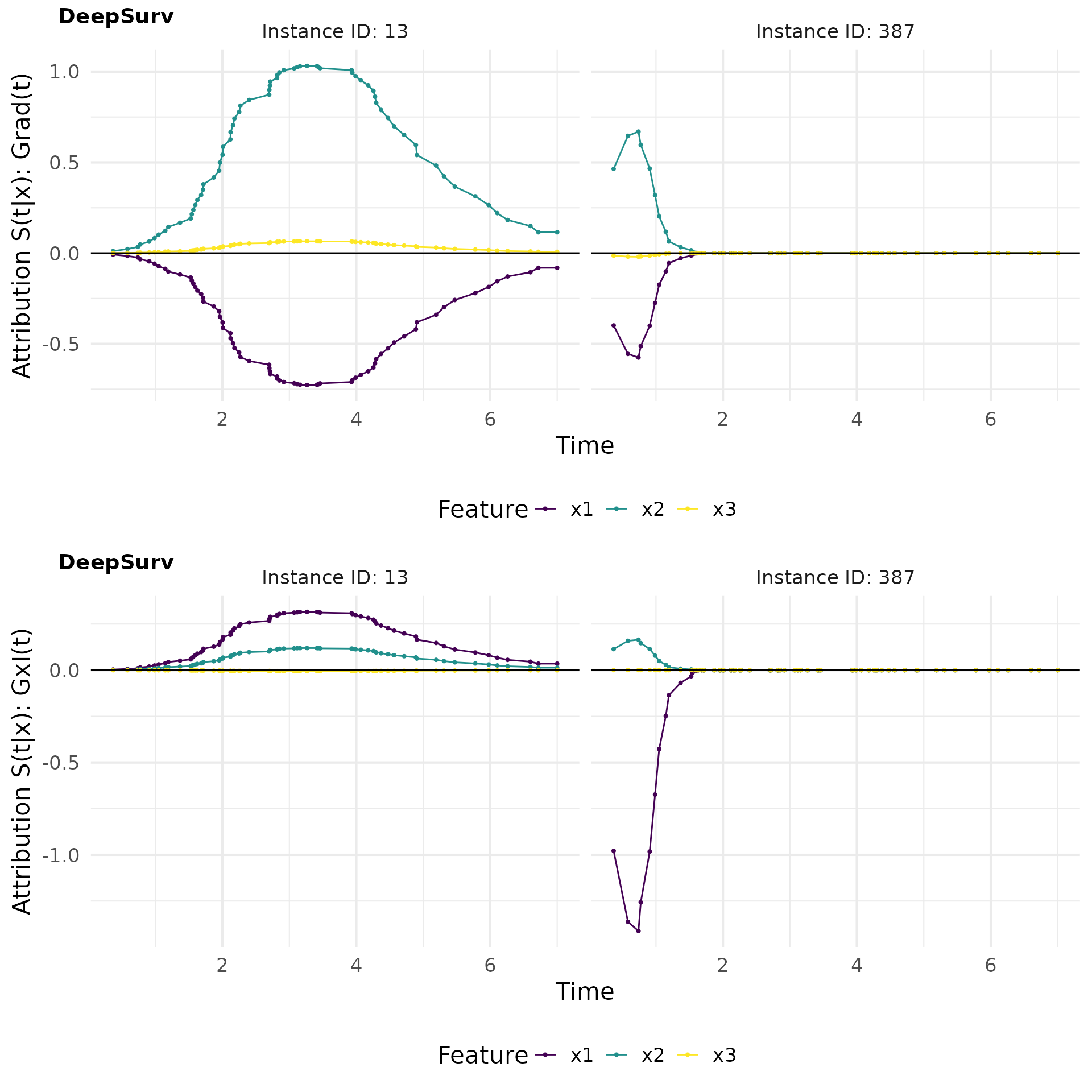

SmoothGrad x I(t)

SmoothGrad x I(t) is a method that adds noise to the input features and computes the average gradient over multiple noisy samples, multiplied by the survival predictions. This approach helps to reduce the noise in the gradient estimates and provides a clearer picture of the feature importance.

# Compute SmoothGradxInput
sgin_cox <- surv_smoothgrad(exp_coxtime, instance = tid_ids, n = 50, noise_level = 0.3,
                          times_input = TRUE)
sgin_deephit <- surv_smoothgrad(exp_deephit, instance = tid_ids, n = 50, noise_level = 0.3,
                              times_input = TRUE)
sgin_deepsurv <- surv_smoothgrad(exp_deepsurv, instance = tid_ids, n = 50, noise_level = 0.3,
                               times_input = TRUE)

# Plot attributions
smoothgradin_plot <- cowplot::plot_grid(
  plot(sgin_cox, type = "attr"), 
  plot(sgin_deephit, type = "attr"), 
  plot(sgin_deepsurv, type = "attr"),
  nrow = 3, labels = c("CoxTime", "DeepHit", "DeepSurv"))
smoothgradin_plot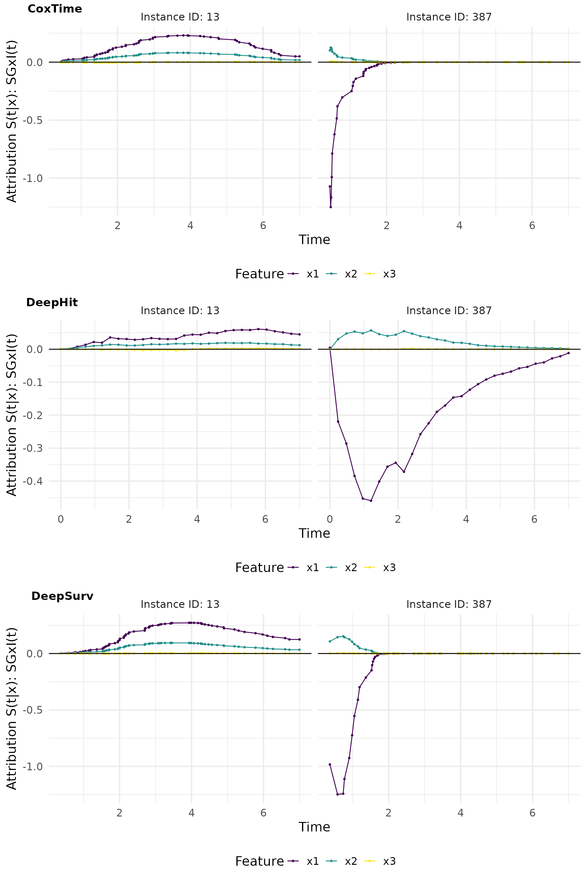

IntGrad(t)

IntGrad(t) is a method that computes the integral of the gradients along a straight line path from a reference point to the input instance. This method provides a more comprehensive view of the feature importance by considering the cumulative effect of the features over time.

Zero baseline

The zero baseline is a reference point where all features are set to zero.

# Compute IntegratedGradient with 0 baseline
x_ref <- matrix(c(0,0,0), nrow = 1)
ig0_cox <- surv_intgrad(exp_coxtime, instance = tid_ids, n = 50, x_ref = x_ref)
ig0_deephit <- surv_intgrad(exp_deephit, instance = tid_ids, n = 50, x_ref = x_ref)
ig0_deepsurv <- surv_intgrad(exp_deepsurv, instance = tid_ids, n = 50, x_ref = x_ref)

# Plot attributions
intgrad0_plot <- cowplot::plot_grid(
  plot(ig0_cox, type = "attr"), 
  plot(ig0_deephit, type = "attr"), 
  plot(ig0_deepsurv, type = "attr"),
  nrow = 3, labels = c("CoxTime", "DeepHit", "DeepSurv"))
intgrad0_plot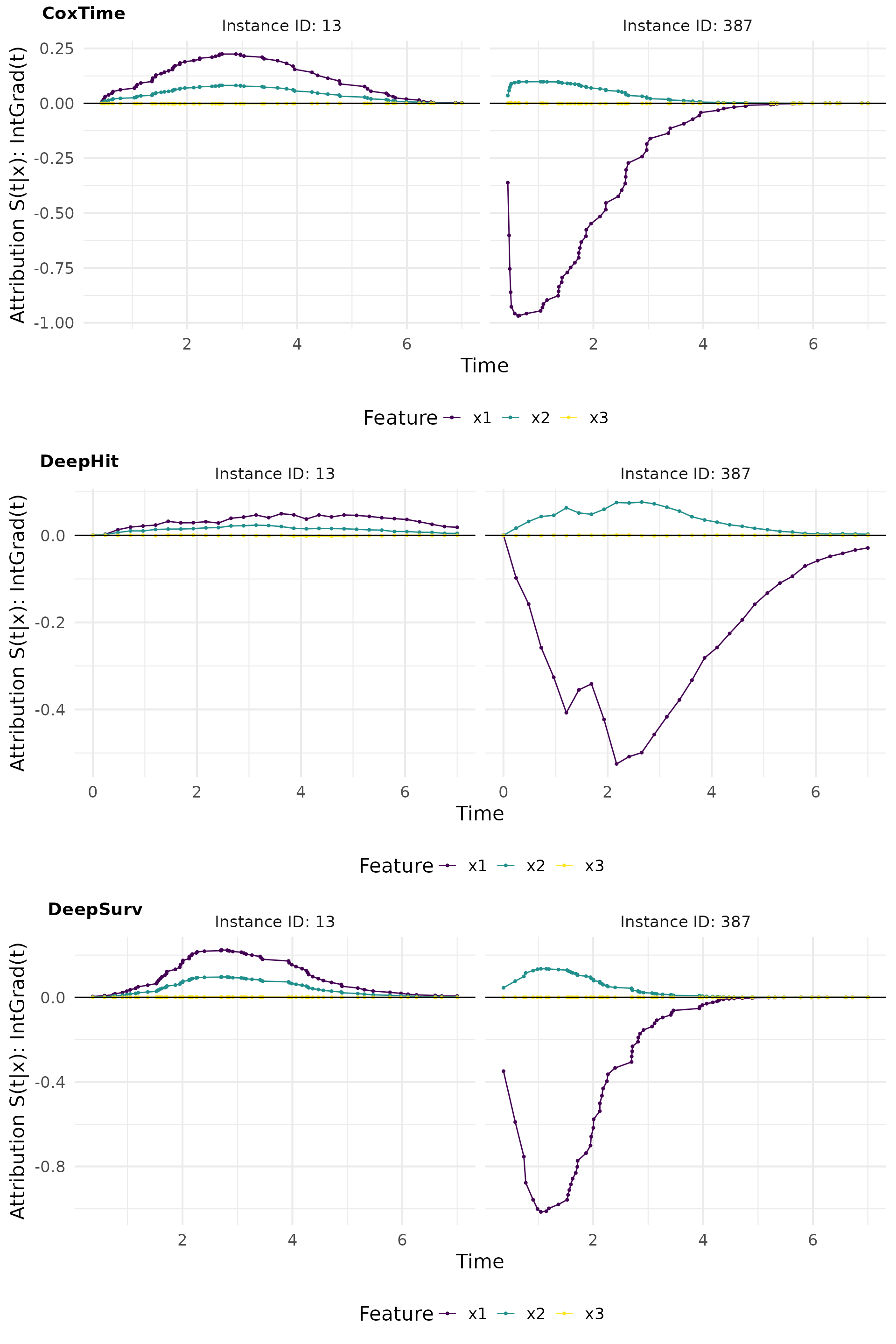

# Plot attributions
intgrad0_plot_comp <- cowplot::plot_grid(
  plot(ig0_cox, add_comp = "all", type = "attr"), 
  plot(ig0_deephit, add_comp = "all", type = "attr"), 
  plot(ig0_deepsurv, add_comp = "all", type = "attr"),
  nrow = 3, labels = c("CoxTime", "DeepHit", "DeepSurv"))
intgrad0_plot_comp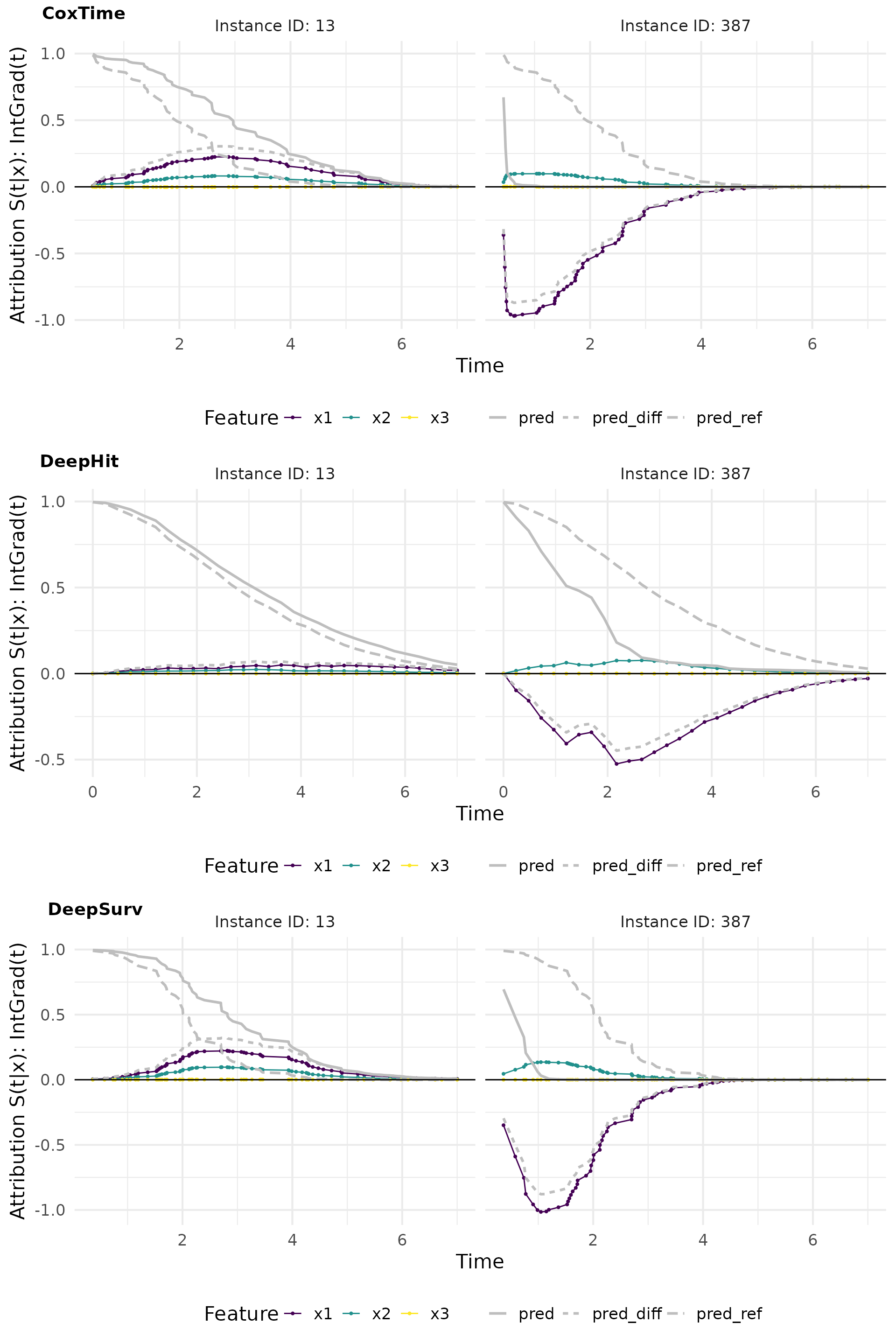

Contribution plots effectively visualize the normalized absolute contribution of each feature to the difference between reference and (survival) prediction over time.

# Plot contributions
intgrad0_plot_contr <- cowplot::plot_grid(
  plot(ig0_cox, type = "contr"), 
  plot(ig0_deephit, type = "contr"), 
  plot(ig0_deepsurv, type = "contr"),
  nrow = 3, labels = c("CoxTime", "DeepHit", "DeepSurv"))
intgrad0_plot_contr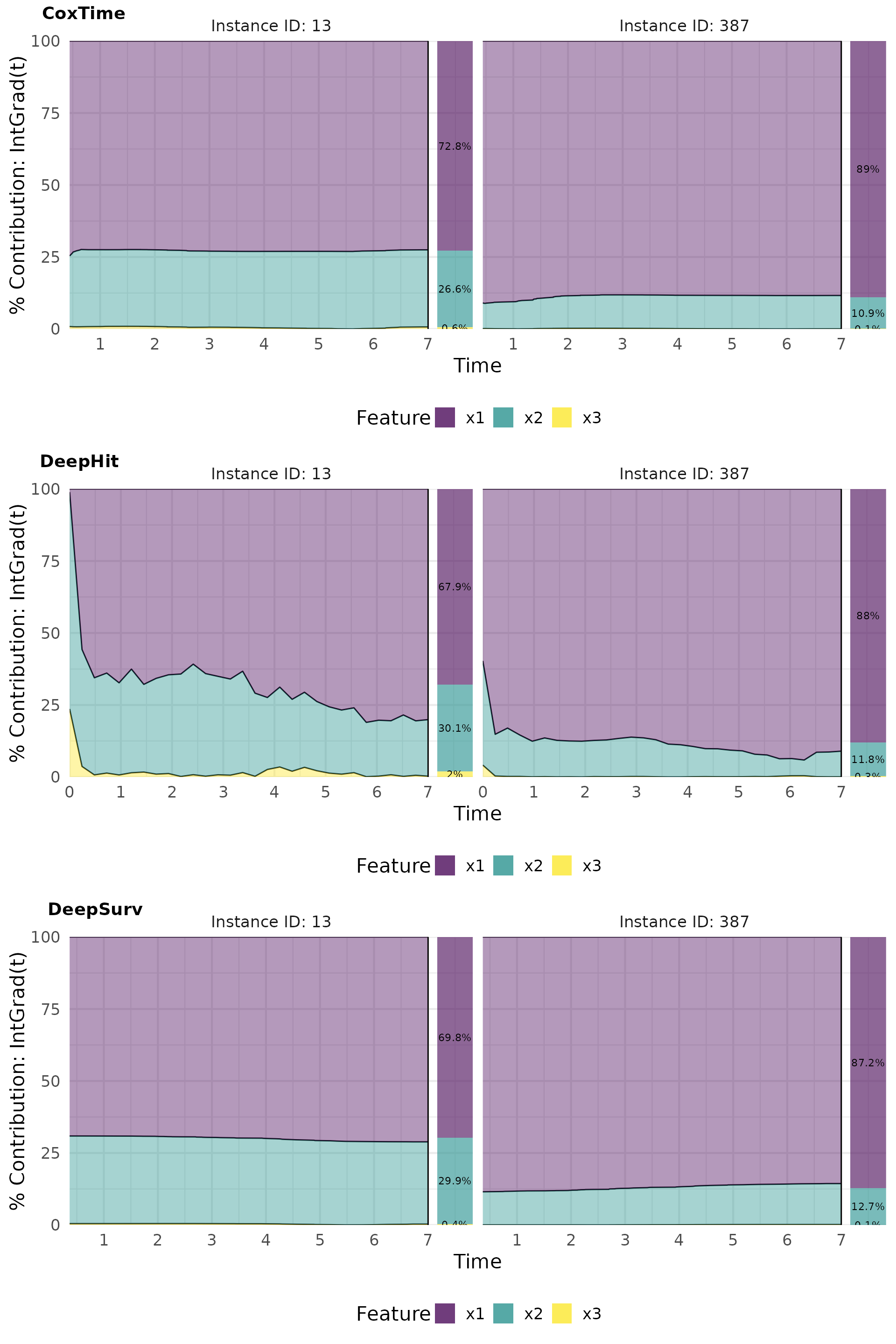

Complementarily, force plots emphasize the relative contribution and direction of each feature at a set of representative survival times.

# Plot force
intgrad0_plot_force <- cowplot::plot_grid(
  plot(ig0_cox, type = "force"),
  plot(ig0_deephit, type = "force"),
  plot(ig0_deepsurv, type = "force"),
  nrow = 3, labels = c("CoxTime", "DeepHit", "DeepSurv"))
intgrad0_plot_force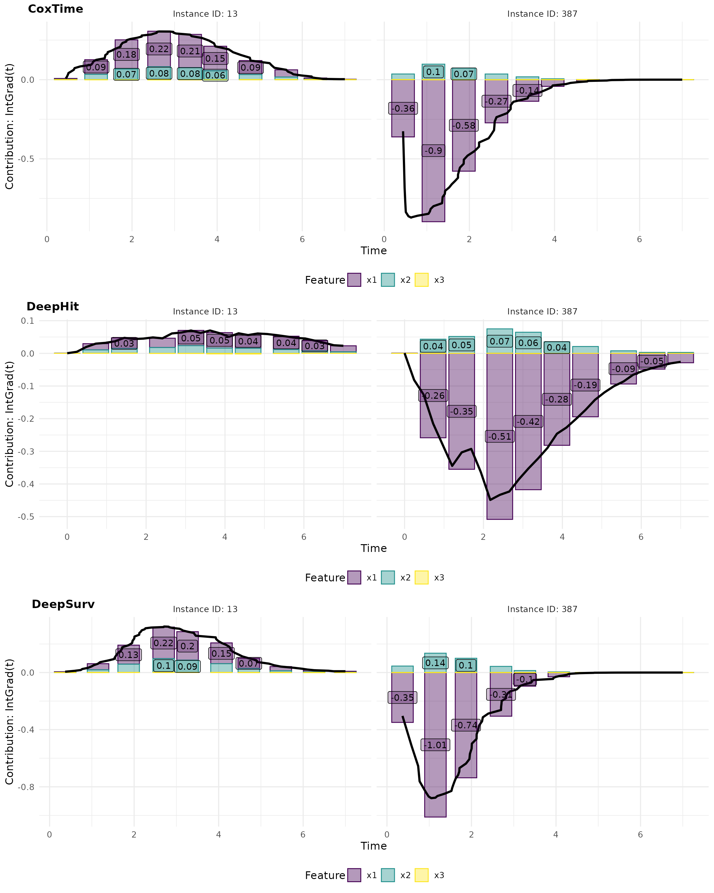

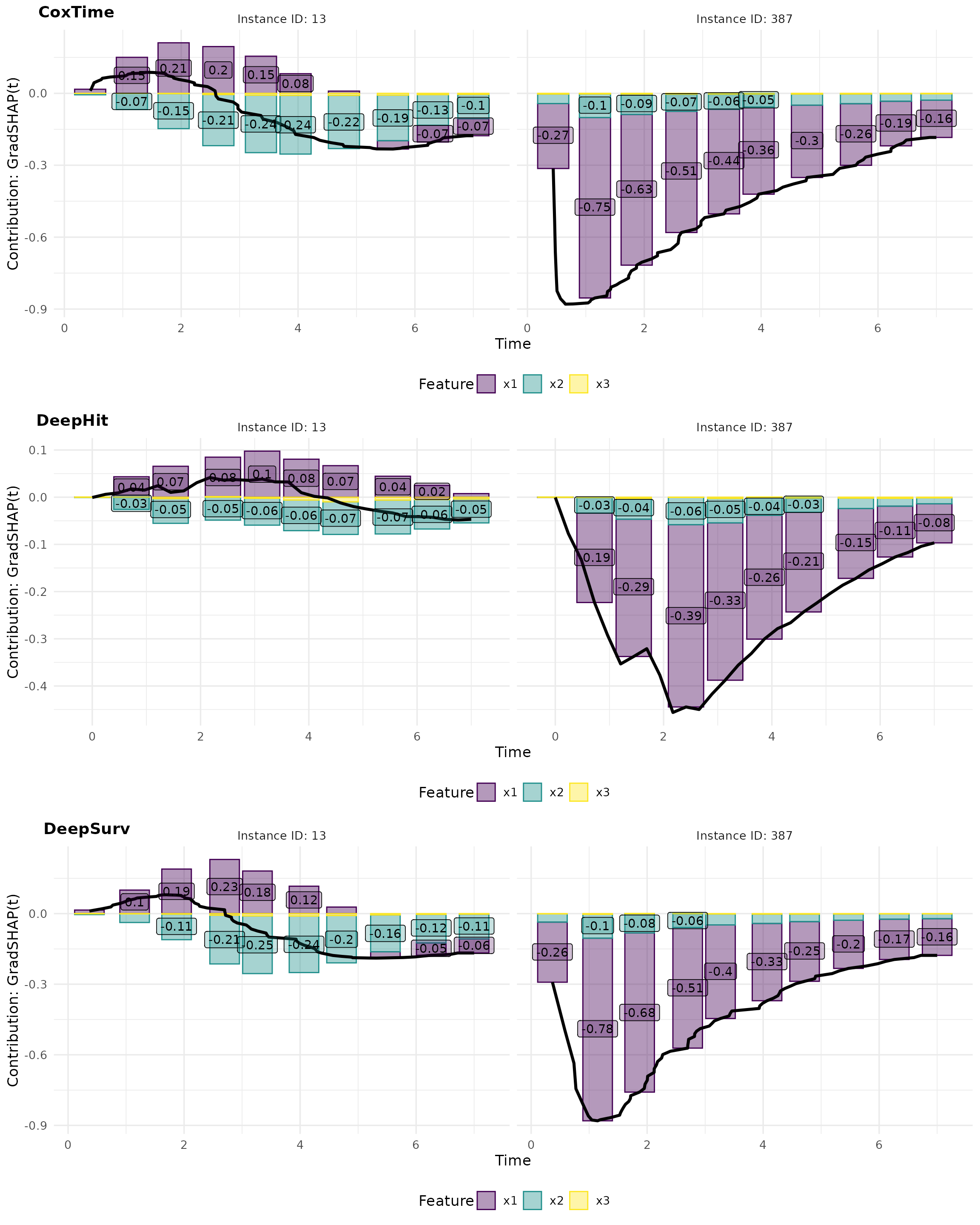
GradSHAP(t)

GradSHAP(t) is a method that computes the SHAP values for survival predictions. It provides a measure of the contribution of each feature to the survival predictions, taking into account the time-dependent effects.

# Compute GradShap
gshap_cox <- surv_gradSHAP(exp_coxtime, instance = tid_ids, n = 50, num_samples = 100)
gshap_deephit <- surv_gradSHAP(exp_deephit, instance = tid_ids, n = 50, num_samples = 100)
gshap_deepsurv <- surv_gradSHAP(exp_deepsurv, instance = tid_ids, n = 50, num_samples = 100)

# Plot attributions
gshap_plot <- cowplot::plot_grid(
  plot(gshap_cox, type = "attr"), 
  plot(gshap_deephit, type = "attr"), 
  plot(gshap_deepsurv, type = "attr"),
  nrow = 3, labels = c("CoxTime", "DeepHit", "DeepSurv"))
gshap_plot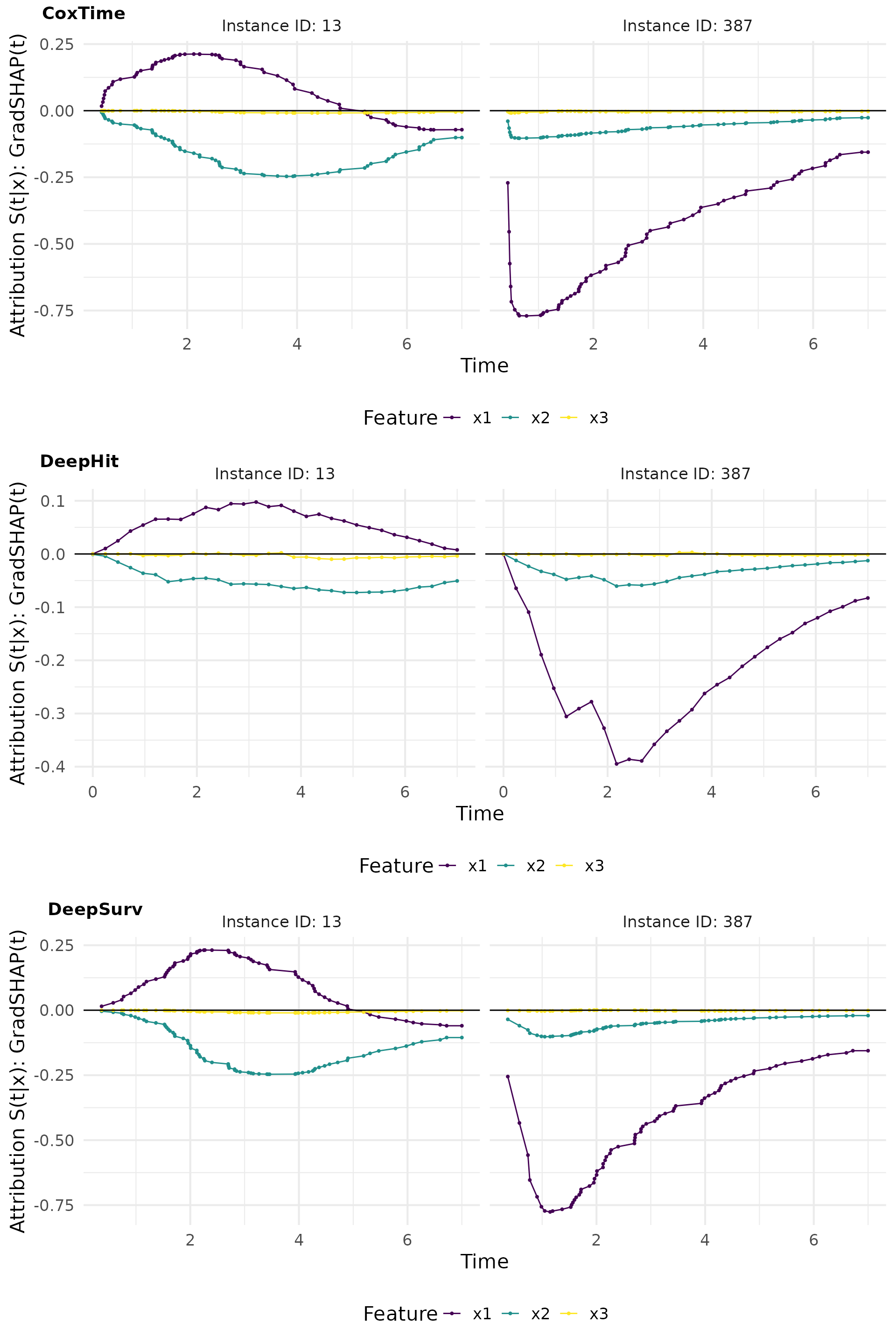

# Plot attributions
gshap_plot_comp <- cowplot::plot_grid(
  plot(gshap_cox, add_comp = "all", type = "attr"), 
  plot(gshap_deephit, add_comp = "all", type = "attr"), 
  plot(gshap_deepsurv, add_comp = "all", type = "attr"),
  nrow = 3, labels = c("CoxTime", "DeepHit", "DeepSurv"))
gshap_plot_comp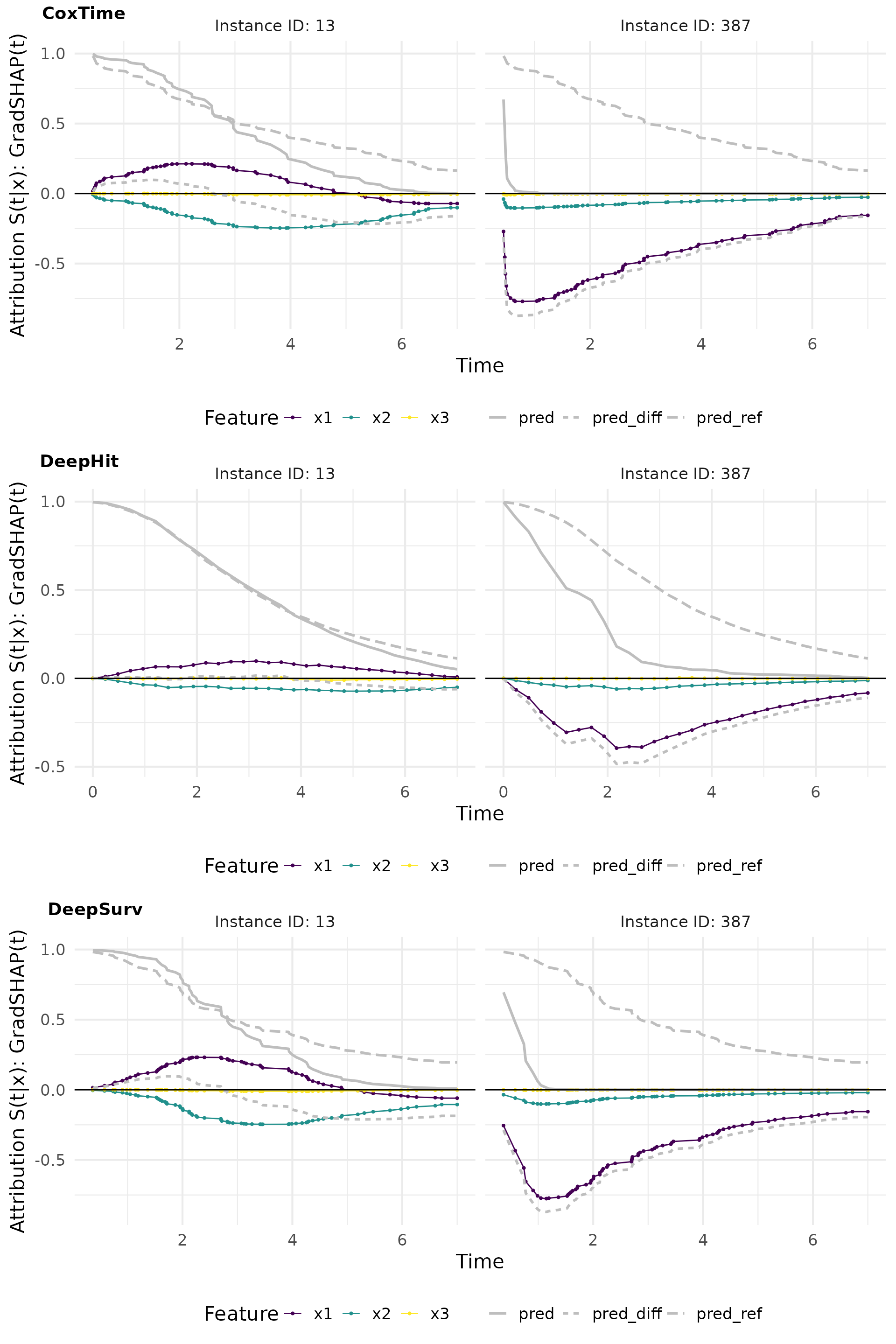

# Plot contributions 
gshap_plot_contr <- cowplot::plot_grid(
  plot(gshap_cox, type = "contr"), 
  plot(gshap_deephit, type = "contr"), 
  plot(gshap_deepsurv, type = "contr"),
  nrow = 3, labels = c("CoxTime", "DeepHit", "DeepSurv"))
gshap_plot_contr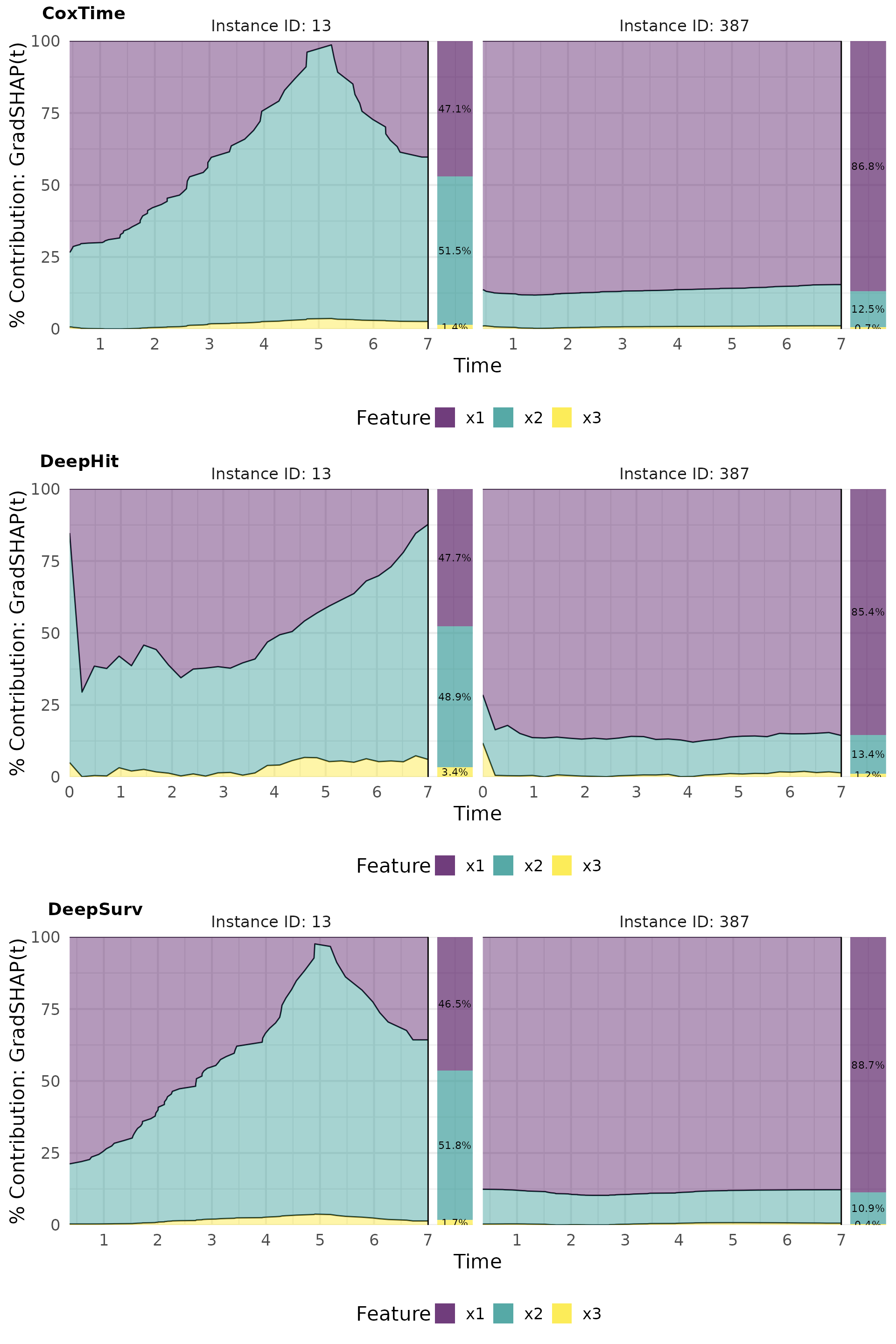

# Plot force
gshap_plot_force <- cowplot::plot_grid(
  plot(gshap_cox, type = "force"), 
  plot(gshap_deephit, type = "force"),
  plot(gshap_deepsurv, type = "force"),
  nrow = 3, labels = c("CoxTime", "DeepHit", "DeepSurv"))
gshap_plot_force