4: The Tidyverse

The Tidyverse is a collection of R packages created and maintained by the same group of people, largely from the same company that also created RStudio: Posit!

The Tidyverse is designed to make data science easier, more efficient, and more fun.
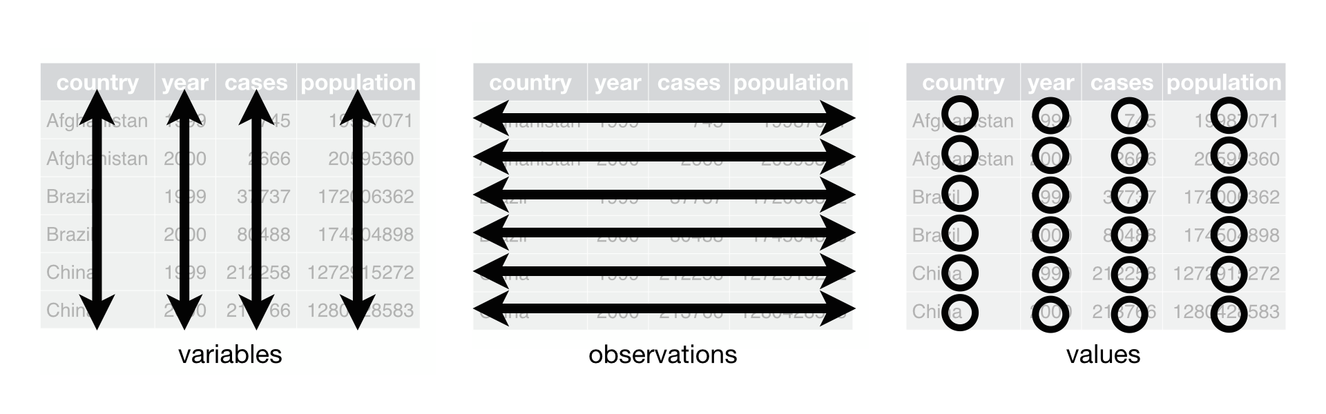
It is built around the idea of tidy data, which in essence just means that data is organized in a way that makes it easy to work with. In the previous section we have already heard the two core properties of tidy data:

Each column of your data is a variable
Each row of your data is an observation

And the tidyverse is created in part to make it easy to get your data in that shape and work with data in that shape. If R in general is a language, then we can think of “tidyverse” as a kind of dialect — it’s still R, but it has a specific context and use case and it is spoken by a community of people roughly doing similar kinds of data analysis.

Let’s start by loading the tidyverse meta-package.

library(tidyverse)

── Attaching core tidyverse packages ──────────────────────── tidyverse 2.0.0 ──
✔ dplyr     1.1.4     ✔ readr     2.1.5
✔ forcats   1.0.0     ✔ stringr   1.5.1
✔ ggplot2   3.5.1     ✔ tibble    3.2.1
✔ lubridate 1.9.4     ✔ tidyr     1.3.1
✔ purrr     1.0.2     
── Conflicts ────────────────────────────────────────── tidyverse_conflicts() ──
✖ dplyr::filter() masks stats::filter()
✖ dplyr::lag()    masks stats::lag()
ℹ Use the conflicted package (<http://conflicted.r-lib.org/>) to force all conflicts to become errors

You’ll see a lot of information there, and that’s nothing to worry about. What happened here is the following:

The tidyverse package’s main purpose is to load other packages, like dplyr, ggplot2, tidyr, … -> These are the actual tidyverse packages that provide the functionality we want!
It warns you about conflicting function names, like filter and lag. There are built-in functions in R of the same name that do very different things than they do in the tidyverse, and for the most part that is not a problem unless you try to use the function filter from the dplyr package but forgot to load dplyr beforehand!

Note that in the tidyverse, the tibble enhances the data.frame!
Tibbles are similar to data.frames, but they look nice and avoid some potentially confusing issues.
For now we don’t need to know more, but fur future reference you should not worry when you encounter a tibble!

Tidyverse Basics: Pipes and Verbs

We start by loading the gapminder package again for its dataset, just like we did before, but now we can glimpse it rather than str it:

library(gapminder)

glimpse(gapminder)

Rows: 1,704
Columns: 6
$ country   <fct> "Afghanistan", "Afghanistan", "Afghanistan", "Afghanistan", …
$ continent <fct> Asia, Asia, Asia, Asia, Asia, Asia, Asia, Asia, Asia, Asia, …
$ year      <int> 1952, 1957, 1962, 1967, 1972, 1977, 1982, 1987, 1992, 1997, …
$ lifeExp   <dbl> 28.801, 30.332, 31.997, 34.020, 36.088, 38.438, 39.854, 40.8…
$ pop       <int> 8425333, 9240934, 10267083, 11537966, 13079460, 14880372, 12…
$ gdpPercap <dbl> 779.4453, 820.8530, 853.1007, 836.1971, 739.9811, 786.1134, …

Remember how it was somewhat awkward to select specific rows and columns from the data.frame before?

For example, here is “country, life expectancy and population for all Asian countries in 1967” in base R syntax:

gapminder[gapminder$continent == "Asia" & gapminder$year == 1967, 
          c("country", "lifeExp", "pop")]

# A tibble: 33 × 3
   country          lifeExp       pop
   <fct>              <dbl>     <int>
 1 Afghanistan         34.0  11537966
 2 Bahrain             59.9    202182
 3 Bangladesh          43.5  62821884
 4 Cambodia            45.4   6960067
 5 China               58.4 754550000
 6 Hong Kong, China    70     3722800
 7 India               47.2 506000000
 8 Indonesia           46.0 109343000
 9 Iran                52.5  26538000
10 Iraq                54.5   8519282
# ℹ 23 more rows

In the tidyverse, or specifically dplyr syntax, we would write it like this:

gapminder |>
  filter(continent == "Asia" & year == 1967) |>
  select(country, lifeExp, pop)

# A tibble: 33 × 3
   country          lifeExp       pop
   <fct>              <dbl>     <int>
 1 Afghanistan         34.0  11537966
 2 Bahrain             59.9    202182
 3 Bangladesh          43.5  62821884
 4 Cambodia            45.4   6960067
 5 China               58.4 754550000
 6 Hong Kong, China    70     3722800
 7 India               47.2 506000000
 8 Indonesia           46.0 109343000
 9 Iran                52.5  26538000
10 Iraq                54.5   8519282
# ℹ 23 more rows

What happened here? Let’s dissect this one by one:

We started with the gapminder dataset, and then, via the “pipe” |>,
We used filter() to select rows using a logical expression, and then
We used select() to select specific columns (without having to quote than with "!)

This is a combination of the pipe-syntax, which passes things down to the next function, and the most common tidyverse verbs that are at the core of most data operations.

The pipe |> works everywhere in R, and x |> foo() is just a different way to write foo(x):

x <- 1:10

length(x)

[1] 10

x |> length()

[1] 10

This becomes really powerful once we chain many functions.
Consider a made-up example:

x |>
  do_the_thing() |>
  do_the_other_thing() |>
  twist_it() |>
  shake_it_around() |>
  do_a_little_dance()

Here you can read the code top to bottom, and understand the sequence of events just by following the code. Consider what this would look like without the |>:

do_a_little_dance(shake_it_around(twist_it(do_the_other_thing(do_the_thing(x)))))

Or, with a little more indentation:

do_a_little_dance(
  shake_it_around(
    twist_it(
      do_the_other_thing(
        do_the_thing(x)
      )
    )
  )
)

You would have to read the code “inside out” to follow what’s happening here.

Another alternative would be to create new variables or overwrite the previous one, like so:

x <- do_the_thing(x)
x <- do_the_other_thing(x)
x <- twist_it(x)
x <- shake_it_around(x) 
x <- do_a_little_dance(x)

The pipe syntax might take some getting used to, but usually people find it quite intuitive after a while.

Please keep in mind though that not everything has to be translated into a pipe-syntax, and that there are always other ways to do the same thing.

Common Verbs (I)

All verbs take a data.frame (or tibble, which are almost the same thing) as their first argument, and the most important ones are:

select(): Selects variables (columns) of the dataset (without quoting them with " ")
filter(): Filters the dataset to only the rows matching the condition(s) inside
arrange(): Sorts the dataset by a variable like pop, optionally in decreasing order by using desc() inside.

We start with select(), which is fairly self-explanatory and corresponds to using [ ] with column names or indices as we’ve seen before

gapminder |>
  select(year, country, pop)

# A tibble: 1,704 × 3
    year country          pop
   <int> <fct>          <int>
 1  1952 Afghanistan  8425333
 2  1957 Afghanistan  9240934
 3  1962 Afghanistan 10267083
 4  1967 Afghanistan 11537966
 5  1972 Afghanistan 13079460
 6  1977 Afghanistan 14880372
 7  1982 Afghanistan 12881816
 8  1987 Afghanistan 13867957
 9  1992 Afghanistan 16317921
10  1997 Afghanistan 22227415
# ℹ 1,694 more rows

# If we happen to know the variable indices, this also works
gapminder |>
  select(3, 1, 5)

# A tibble: 1,704 × 3
    year country          pop
   <int> <fct>          <int>
 1  1952 Afghanistan  8425333
 2  1957 Afghanistan  9240934
 3  1962 Afghanistan 10267083
 4  1967 Afghanistan 11537966
 5  1972 Afghanistan 13079460
 6  1977 Afghanistan 14880372
 7  1982 Afghanistan 12881816
 8  1987 Afghanistan 13867957
 9  1992 Afghanistan 16317921
10  1997 Afghanistan 22227415
# ℹ 1,694 more rows

In cases where we pick out individual variables, we often want to sort by one as well:

gapminder |>
  select(year, continent, country) |>
  arrange(year)

# A tibble: 1,704 × 3
    year continent country    
   <int> <fct>     <fct>      
 1  1952 Asia      Afghanistan
 2  1952 Europe    Albania    
 3  1952 Africa    Algeria    
 4  1952 Africa    Angola     
 5  1952 Americas  Argentina  
 6  1952 Oceania   Australia  
 7  1952 Europe    Austria    
 8  1952 Asia      Bahrain    
 9  1952 Asia      Bangladesh 
10  1952 Europe    Belgium    
# ℹ 1,694 more rows

Or sorting descendingly with the desc() helper function:

gapminder |>
  select(year, continent, country) |>
  arrange(desc(year))

# A tibble: 1,704 × 3
    year continent country    
   <int> <fct>     <fct>      
 1  2007 Asia      Afghanistan
 2  2007 Europe    Albania    
 3  2007 Africa    Algeria    
 4  2007 Africa    Angola     
 5  2007 Americas  Argentina  
 6  2007 Oceania   Australia  
 7  2007 Europe    Austria    
 8  2007 Asia      Bahrain    
 9  2007 Asia      Bangladesh 
10  2007 Europe    Belgium    
# ℹ 1,694 more rows

For a numeric variable like year we could also just sort by a negative of the variable:

gapminder |>
  select(year, continent, country) |>
  arrange(-year)

# A tibble: 1,704 × 3
    year continent country    
   <int> <fct>     <fct>      
 1  2007 Asia      Afghanistan
 2  2007 Europe    Albania    
 3  2007 Africa    Algeria    
 4  2007 Africa    Angola     
 5  2007 Americas  Argentina  
 6  2007 Oceania   Australia  
 7  2007 Europe    Austria    
 8  2007 Asia      Bahrain    
 9  2007 Asia      Bangladesh 
10  2007 Europe    Belgium    
# ℹ 1,694 more rows

But desc() has the benefit of also working for character (sorted alphabetically) or factor variables (sorted by their levels), which makes desc() applicable in more cases.

gapminder |>
  select(year, continent, country) |>
  arrange(desc(continent))

# A tibble: 1,704 × 3
    year continent country  
   <int> <fct>     <fct>    
 1  1952 Oceania   Australia
 2  1957 Oceania   Australia
 3  1962 Oceania   Australia
 4  1967 Oceania   Australia
 5  1972 Oceania   Australia
 6  1977 Oceania   Australia
 7  1982 Oceania   Australia
 8  1987 Oceania   Australia
 9  1992 Oceania   Australia
10  1997 Oceania   Australia
# ℹ 1,694 more rows

gapminder97 <- gapminder |>
  filter(year == 1997) |>
  arrange(pop)

Note that in filter() you use logical expressions as we’ve seen in section 2!
You can combine multiple conditions by passing them as separate arguments with , which inside filter() is the same as using the logical AND with &:

# Explicitly using AND & to combine year and country conditions
gapminder |>
  filter(year == 1997 & country == "Iceland")

# A tibble: 1 × 6
  country continent  year lifeExp    pop gdpPercap
  <fct>   <fct>     <int>   <dbl>  <int>     <dbl>
1 Iceland Europe     1997    79.0 271192    28061.

# Identical:
gapminder |>
  filter(
    year > 1990, 
    country == "Iceland"
  )

# A tibble: 4 × 6
  country continent  year lifeExp    pop gdpPercap
  <fct>   <fct>     <int>   <dbl>  <int>     <dbl>
1 Iceland Europe     1992    78.8 259012    25144.
2 Iceland Europe     1997    79.0 271192    28061.
3 Iceland Europe     2002    80.5 288030    31163.
4 Iceland Europe     2007    81.8 301931    36181.

As a more advanced example, we can use select()-helper functions to select variables that start with a certain pattern or contain a certain word:

gapminder |>
  select(starts_with("c"))

# A tibble: 1,704 × 2
   country     continent
   <fct>       <fct>    
 1 Afghanistan Asia     
 2 Afghanistan Asia     
 3 Afghanistan Asia     
 4 Afghanistan Asia     
 5 Afghanistan Asia     
 6 Afghanistan Asia     
 7 Afghanistan Asia     
 8 Afghanistan Asia     
 9 Afghanistan Asia     
10 Afghanistan Asia     
# ℹ 1,694 more rows

gapminder |>
  select(contains("gdp"))

# A tibble: 1,704 × 1
   gdpPercap
       <dbl>
 1      779.
 2      821.
 3      853.
 4      836.
 5      740.
 6      786.
 7      978.
 8      852.
 9      649.
10      635.
# ℹ 1,694 more rows

gapminder |>
  select(ends_with("p"))

# A tibble: 1,704 × 3
   lifeExp      pop gdpPercap
     <dbl>    <int>     <dbl>
 1    28.8  8425333      779.
 2    30.3  9240934      821.
 3    32.0 10267083      853.
 4    34.0 11537966      836.
 5    36.1 13079460      740.
 6    38.4 14880372      786.
 7    39.9 12881816      978.
 8    40.8 13867957      852.
 9    41.7 16317921      649.
10    41.8 22227415      635.
# ℹ 1,694 more rows

Your turn

Select the country and life expectancy variables for the year 1952
Subset the dataset to only contain data recorded after 1990
Subset the dataset to only contain data in the 1970s for Ecuador

gapminder |>
  filter(year == 1952) |>
  select(country, lifeExp)

# A tibble: 142 × 2
   country     lifeExp
   <fct>         <dbl>
 1 Afghanistan    28.8
 2 Albania        55.2
 3 Algeria        43.1
 4 Angola         30.0
 5 Argentina      62.5
 6 Australia      69.1
 7 Austria        66.8
 8 Bahrain        50.9
 9 Bangladesh     37.5
10 Belgium        68  
# ℹ 132 more rows

gapminder |>
  filter(year > 1990)

# A tibble: 568 × 6
   country     continent  year lifeExp      pop gdpPercap
   <fct>       <fct>     <int>   <dbl>    <int>     <dbl>
 1 Afghanistan Asia       1992    41.7 16317921      649.
 2 Afghanistan Asia       1997    41.8 22227415      635.
 3 Afghanistan Asia       2002    42.1 25268405      727.
 4 Afghanistan Asia       2007    43.8 31889923      975.
 5 Albania     Europe     1992    71.6  3326498     2497.
 6 Albania     Europe     1997    73.0  3428038     3193.
 7 Albania     Europe     2002    75.7  3508512     4604.
 8 Albania     Europe     2007    76.4  3600523     5937.
 9 Algeria     Africa     1992    67.7 26298373     5023.
10 Algeria     Africa     1997    69.2 29072015     4797.
# ℹ 558 more rows

gapminder |>
  filter(
    year >= 1970, year <= 1979,
    country == "Ecuador"
  )

# A tibble: 2 × 6
  country continent  year lifeExp     pop gdpPercap
  <fct>   <fct>     <int>   <dbl>   <int>     <dbl>
1 Ecuador Americas   1972    58.8 6298651     5281.
2 Ecuador Americas   1977    61.3 7278866     6680.

gapminder |> 
  filter(year > 1969 & year < 1980) |> 
  filter(country == "Ecuador")

# A tibble: 2 × 6
  country continent  year lifeExp     pop gdpPercap
  <fct>   <fct>     <int>   <dbl>   <int>     <dbl>
1 Ecuador Americas   1972    58.8 6298651     5281.
2 Ecuador Americas   1977    61.3 7278866     6680.

gapminder |>
  filter(
    between(year, 1970, 1979),
    country == "Ecuador"
  )

# A tibble: 2 × 6
  country continent  year lifeExp     pop gdpPercap
  <fct>   <fct>     <int>   <dbl>   <int>     <dbl>
1 Ecuador Americas   1972    58.8 6298651     5281.
2 Ecuador Americas   1977    61.3 7278866     6680.

Hint: When you select and filter, keep in mind the order of operations!
You can’t filter by a variable which you have de-selected beforehand.

Common Verbs (II)

So far we have only selected specific subsets of our data, but now we want to actually do something! For that, we have two main options:

Creating a new variable
Calculating some summary statistic like the mean or median

mutate(): Creates a new variables, e.g. create pop_m as the variable pop divided by 1,000,000
summarize(): Often used together with group_by(), this summarizes the dataset by calculating something for each group declared by group_by()
group_by(): Declares the dataset to be grouped by the values of variable like continent – we will see examples next!

gapminder <- gapminder |>
  mutate(pop_m = pop / 1e6)

gapminder |>
  mutate(pop = pop / 1e6)

# A tibble: 1,704 × 7
   country     continent  year lifeExp   pop gdpPercap pop_m
   <fct>       <fct>     <int>   <dbl> <dbl>     <dbl> <dbl>
 1 Afghanistan Asia       1952    28.8  8.43      779.  8.43
 2 Afghanistan Asia       1957    30.3  9.24      821.  9.24
 3 Afghanistan Asia       1962    32.0 10.3       853. 10.3 
 4 Afghanistan Asia       1967    34.0 11.5       836. 11.5 
 5 Afghanistan Asia       1972    36.1 13.1       740. 13.1 
 6 Afghanistan Asia       1977    38.4 14.9       786. 14.9 
 7 Afghanistan Asia       1982    39.9 12.9       978. 12.9 
 8 Afghanistan Asia       1987    40.8 13.9       852. 13.9 
 9 Afghanistan Asia       1992    41.7 16.3       649. 16.3 
10 Afghanistan Asia       1997    41.8 22.2       635. 22.2 
# ℹ 1,694 more rows

gapminder |>
  mutate(pop_mean = mean(pop))

# A tibble: 1,704 × 8
   country     continent  year lifeExp      pop gdpPercap pop_m  pop_mean
   <fct>       <fct>     <int>   <dbl>    <int>     <dbl> <dbl>     <dbl>
 1 Afghanistan Asia       1952    28.8  8425333      779.  8.43 29601212.
 2 Afghanistan Asia       1957    30.3  9240934      821.  9.24 29601212.
 3 Afghanistan Asia       1962    32.0 10267083      853. 10.3  29601212.
 4 Afghanistan Asia       1967    34.0 11537966      836. 11.5  29601212.
 5 Afghanistan Asia       1972    36.1 13079460      740. 13.1  29601212.
 6 Afghanistan Asia       1977    38.4 14880372      786. 14.9  29601212.
 7 Afghanistan Asia       1982    39.9 12881816      978. 12.9  29601212.
 8 Afghanistan Asia       1987    40.8 13867957      852. 13.9  29601212.
 9 Afghanistan Asia       1992    41.7 16317921      649. 16.3  29601212.
10 Afghanistan Asia       1997    41.8 22227415      635. 22.2  29601212.
# ℹ 1,694 more rows

gapminder |>
  summarize(
    pop_mean = mean(pop)
  )

# A tibble: 1 × 1
   pop_mean
      <dbl>
1 29601212.

gapminder |>
  group_by(continent)

# A tibble: 1,704 × 7
# Groups:   continent [5]
   country     continent  year lifeExp      pop gdpPercap pop_m
   <fct>       <fct>     <int>   <dbl>    <int>     <dbl> <dbl>
 1 Afghanistan Asia       1952    28.8  8425333      779.  8.43
 2 Afghanistan Asia       1957    30.3  9240934      821.  9.24
 3 Afghanistan Asia       1962    32.0 10267083      853. 10.3 
 4 Afghanistan Asia       1967    34.0 11537966      836. 11.5 
 5 Afghanistan Asia       1972    36.1 13079460      740. 13.1 
 6 Afghanistan Asia       1977    38.4 14880372      786. 14.9 
 7 Afghanistan Asia       1982    39.9 12881816      978. 12.9 
 8 Afghanistan Asia       1987    40.8 13867957      852. 13.9 
 9 Afghanistan Asia       1992    41.7 16317921      649. 16.3 
10 Afghanistan Asia       1997    41.8 22227415      635. 22.2 
# ℹ 1,694 more rows

gapminder |>
  group_by(continent) |>
  summarize(mean_pop = mean(pop))

# A tibble: 5 × 2
  continent  mean_pop
  <fct>         <dbl>
1 Africa     9916003.
2 Americas  24504795.
3 Asia      77038722.
4 Europe    17169765.
5 Oceania    8874672.

Or multiple things combined:

gapminder |>
  filter(year >= 1980) |>
  mutate(pop_m = pop / 1e6) |>
  group_by(continent) |>
  summarize(
    mean_pop_m = mean(pop_m),
    median_pop_m = median(pop_m),
    min_pop_m = min(pop_m),
    max_pop_m = max(pop_m)
  )

# A tibble: 5 × 5
  continent mean_pop_m median_pop_m min_pop_m max_pop_m
  <fct>          <dbl>        <dbl>     <dbl>     <dbl>
1 Africa          13.6         7.10    0.0986     135. 
2 Americas        30.7         8.18    1.06       301. 
3 Asia            98.0        19.7     0.378     1319. 
4 Europe          18.7         9.03    0.234       82.4
5 Oceania         10.8         9.65    3.21        20.4

Your turn

install the tidyverse & load with library(tidyverse)
Explain in words what has happened in the previous code chunk.
What happens if you use summarize() without group_by()?
Use summarise() and the helpful n_distinct() to calculate the number of countries per continent
Create a new variable gdpPercap_m as the variable gdpPercap divided by 1 Million and rounded to 2 decimal places

gapminder |>
  group_by(continent) |>
  summarize(
    num_countries = n_distinct(country),
    n = n()
  )

# A tibble: 5 × 3
  continent num_countries     n
  <fct>             <int> <int>
1 Africa               52   624
2 Americas             25   300
3 Asia                 33   396
4 Europe               30   360
5 Oceania               2    24

gapminder |>
  filter(continent == "Oceania") |>
  group_by(country) |>
  summarize(
    n = n(),
    num_years = n_distinct(year)
  )

# A tibble: 2 × 3
  country         n num_years
  <fct>       <int>     <int>
1 Australia      12        12
2 New Zealand    12        12

gapminder |>
  mutate(gdpPercap_m = round(gdpPercap / 1e3, digits = 2))

# A tibble: 1,704 × 8
   country     continent  year lifeExp      pop gdpPercap pop_m gdpPercap_m
   <fct>       <fct>     <int>   <dbl>    <int>     <dbl> <dbl>       <dbl>
 1 Afghanistan Asia       1952    28.8  8425333      779.  8.43        0.78
 2 Afghanistan Asia       1957    30.3  9240934      821.  9.24        0.82
 3 Afghanistan Asia       1962    32.0 10267083      853. 10.3         0.85
 4 Afghanistan Asia       1967    34.0 11537966      836. 11.5         0.84
 5 Afghanistan Asia       1972    36.1 13079460      740. 13.1         0.74
 6 Afghanistan Asia       1977    38.4 14880372      786. 14.9         0.79
 7 Afghanistan Asia       1982    39.9 12881816      978. 12.9         0.98
 8 Afghanistan Asia       1987    40.8 13867957      852. 13.9         0.85
 9 Afghanistan Asia       1992    41.7 16317921      649. 16.3         0.65
10 Afghanistan Asia       1997    41.8 22227415      635. 22.2         0.64
# ℹ 1,694 more rows

gapminder |>
  mutate(gdpPercap_m = gdpPercap / 1e6) |>
  mutate(gdpPercap_m = round(gdpPercap_m, digits = 2))

# A tibble: 1,704 × 8
   country     continent  year lifeExp      pop gdpPercap pop_m gdpPercap_m
   <fct>       <fct>     <int>   <dbl>    <int>     <dbl> <dbl>       <dbl>
 1 Afghanistan Asia       1952    28.8  8425333      779.  8.43           0
 2 Afghanistan Asia       1957    30.3  9240934      821.  9.24           0
 3 Afghanistan Asia       1962    32.0 10267083      853. 10.3            0
 4 Afghanistan Asia       1967    34.0 11537966      836. 11.5            0
 5 Afghanistan Asia       1972    36.1 13079460      740. 13.1            0
 6 Afghanistan Asia       1977    38.4 14880372      786. 14.9            0
 7 Afghanistan Asia       1982    39.9 12881816      978. 12.9            0
 8 Afghanistan Asia       1987    40.8 13867957      852. 13.9            0
 9 Afghanistan Asia       1992    41.7 16317921      649. 16.3            0
10 Afghanistan Asia       1997    41.8 22227415      635. 22.2            0
# ℹ 1,694 more rows

Other Useful Verbs

Changing Shapes

A more advanced topic but often needed for data manipulation is reshaping your data using the tidyr package.

This might be best explained by example.
Say we want to calculate the difference in life expectancy between 1952 and 2007 for each country and continent, but using the verbs we’ve seen so far we can’t do that with a simple mutate(). We can instead use pivot_wider() which is a function that takes a “long” dataset and pivots it into a “wide” dataset:

gapminder |>
  filter(year %in% c(1952, 2007)) |>
  pivot_wider(
    id_cols = c(country, continent), 
    names_from = year, 
    values_from = lifeExp,
    names_prefix = "lifeExp_"
  ) |>
  mutate(change_life_exp = lifeExp_2007 - lifeExp_1952)

# A tibble: 142 × 5
   country     continent lifeExp_1952 lifeExp_2007 change_life_exp
   <fct>       <fct>            <dbl>        <dbl>           <dbl>
 1 Afghanistan Asia              28.8         43.8            15.0
 2 Albania     Europe            55.2         76.4            21.2
 3 Algeria     Africa            43.1         72.3            29.2
 4 Angola      Africa            30.0         42.7            12.7
 5 Argentina   Americas          62.5         75.3            12.8
 6 Australia   Oceania           69.1         81.2            12.1
 7 Austria     Europe            66.8         79.8            13.0
 8 Bahrain     Asia              50.9         75.6            24.7
 9 Bangladesh  Asia              37.5         64.1            26.6
10 Belgium     Europe            68           79.4            11.4
# ℹ 132 more rows

Combining Things

Sometimes it’s useful to combined datasets by rows or columns:

bind_rows() is for rows, similar to base R’s rbind() but has some advantages

gapminder52 <- gapminder |>
  filter(year == 1952)

gapminder07 <- gapminder |>
  filter(year == 2007)

bind_rows(gapminder52, gapminder07)

# A tibble: 284 × 7
   country     continent  year lifeExp      pop gdpPercap  pop_m
   <fct>       <fct>     <int>   <dbl>    <int>     <dbl>  <dbl>
 1 Afghanistan Asia       1952    28.8  8425333      779.  8.43 
 2 Albania     Europe     1952    55.2  1282697     1601.  1.28 
 3 Algeria     Africa     1952    43.1  9279525     2449.  9.28 
 4 Angola      Africa     1952    30.0  4232095     3521.  4.23 
 5 Argentina   Americas   1952    62.5 17876956     5911. 17.9  
 6 Australia   Oceania    1952    69.1  8691212    10040.  8.69 
 7 Austria     Europe     1952    66.8  6927772     6137.  6.93 
 8 Bahrain     Asia       1952    50.9   120447     9867.  0.120
 9 Bangladesh  Asia       1952    37.5 46886859      684. 46.9  
10 Belgium     Europe     1952    68    8730405     8343.  8.73 
# ℹ 274 more rows

bind_cols() combined datasets by columns, similar to base R’s cbind().
For example, here is a way to create to year-specific variables similar to the pivot_wider() example above

gapminder52 <- gapminder |>
  filter(year == 1952) |>
  rename(lifeExp_1952 = lifeExp)

gapminder07 <- gapminder |>
  filter(year == 2007) |>
  select(lifeExp) |>
  rename(lifeExp_2007 = lifeExp)

bind_cols(gapminder52, gapminder07) |>
  select(starts_with("lifeExp"))

# A tibble: 142 × 2
   lifeExp_1952 lifeExp_2007
          <dbl>        <dbl>
 1         28.8         43.8
 2         55.2         76.4
 3         43.1         72.3
 4         30.0         42.7
 5         62.5         75.3
 6         69.1         81.2
 7         66.8         79.8
 8         50.9         75.6
 9         37.5         64.1
10         68           79.4
# ℹ 132 more rows