2: R Fundamentals

Hello There!

This is a Quarto document. It contains regular text, code, and output when viewed in RStudio. It can also be converted into an HTML (or PDF) document, where code and output are shown together as well.

This text is formatted using Markdown, a lightweight syntax that uses asterisks (*), underscores (_), hyphens (-), and parentheses / brackets (() and []) to format text. We can also embed images:

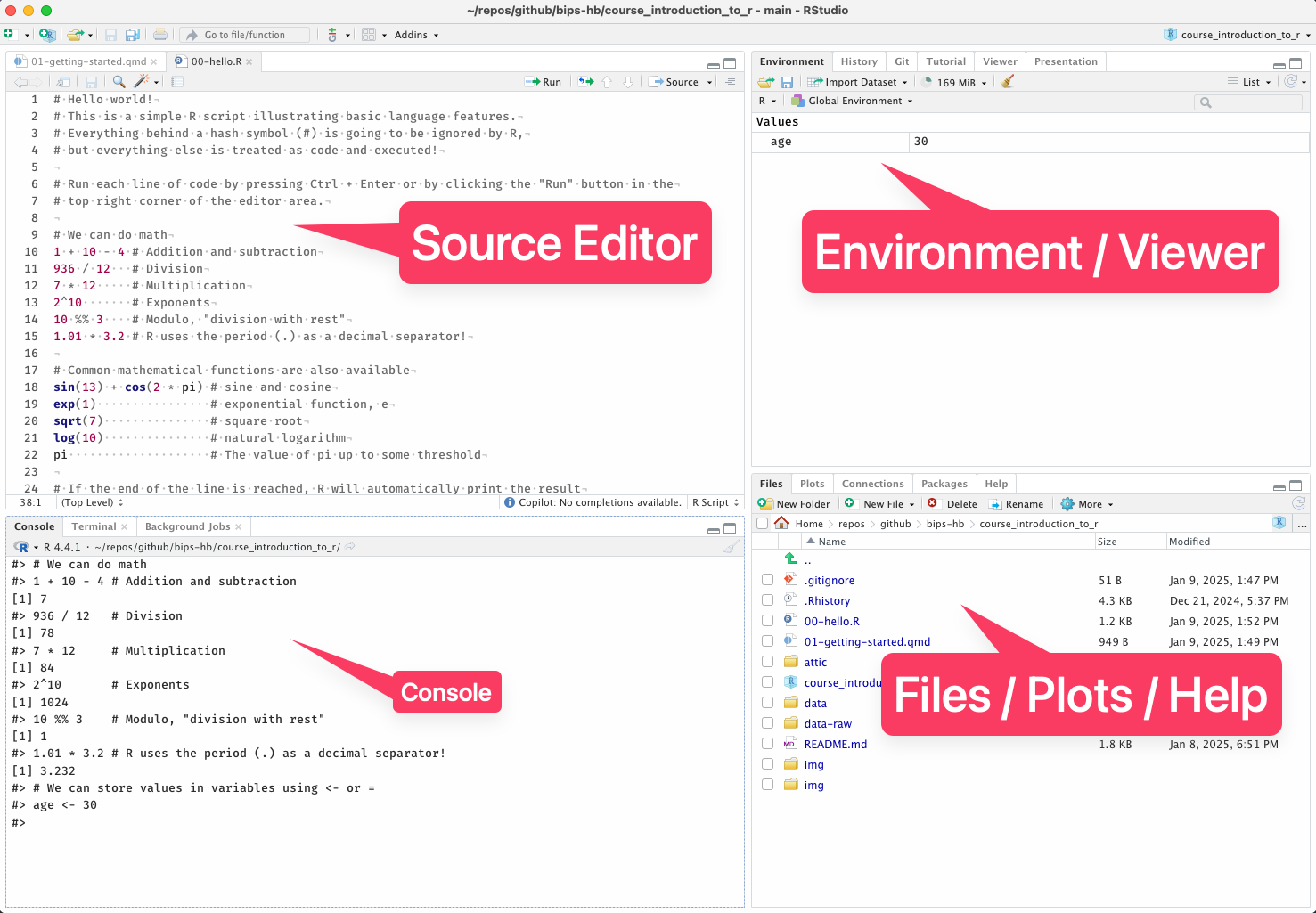
We can also write R code in a code block and execute it using either Ctrl + R like in a regular script or using the green button on the top right of the cell:

# Hello
10 * 5.3

[1] 53

-5 + 10

[1] 5

9^2

[1] 81

2 + 5 / 4

[1] 3.25

(2 + 5) / 4

[1] 1.75

Throughout the workshop, we will use this format to interweave text and explanations with code examples. You can modify the code in the blocks and rerun them to see the results, and later we will provide partial code examples where your task will be to complete them to solve a given task.

Before we try to do any data analysis, we first need to familiarize ourselves with R to know our way around!

In the example script 01-hello.R we have already seen that R can be used like a big calculator, and that’s already pretty useful. For now, we’ll build on that a little.

Variables and Vectors

We have seen how to assign values to a variable, such as age <- 30. This allows us to re-use data and give it a meaningful(!) name in our work. It becomes more useful when we store not just individual number (scalars), but vectors of data.

For example, say we have a small group of patients want to store their basic data, starting with their age:

age <- c(30, 33, 31, 29, 40)

age

[1] 30 33 31 29 40

Now age is a vector, and in R this is the most common type of data structure we deal with. Note that in R, even single numbers like 5 are treated like vectors (of length 1)!

We can use vectors almost exactly like single numbers for basic math:

age + 5

[1] 35 38 36 34 45

age - 10

[1] 20 23 21 19 30

age * 4

[1] 120 132 124 116 160

age / 5

[1] 6.0 6.6 6.2 5.8 8.0

age^2

[1]  900 1089  961  841 1600

What R here is doing is a form of vectorization, by using each element of the vector for the calculation and returning another vector.

We can also conveniently create sequences of numbers using the colon notation :

# 1 through 10
1:10

 [1]  1  2  3  4  5  6  7  8  9 10

# -5 through 5
-5:5

 [1] -5 -4 -3 -2 -1  0  1  2  3  4  5

If we add vectors of the same length, R will try to add each element separately:

age

[1] 30 33 31 29 40

# Same length: ok
age + 1:5

[1] 31 35 34 33 45

# not same length: not ok
age + 1:7

Warning in age + 1:7: longer object length is not a multiple of shorter object
length

[1] 31 35 34 33 45 36 40

But what happens here?

age + 1:10

 [1] 31 35 34 33 45 36 40 39 38 50

This is called recycling and can be great or introduce unexpected behavior if it happens by accident!

A simpler example:

x <- c(5, 5, 5, 5, 5, 5)
x + c(-1, 1)

[1] 4 6 4 6 4 6

Your turn: Creating vectors & variables

Create a vector containing the letters “A”, “B”, “C”, “D”.
Create a vector containing the decimal numbers 1.2, 4.7, 9.4.
Create a vector containing the integers from 10 to 1 in descending order and without writing out the elements.
Create a vector containing a sequence from 10 to 40 in steps of 10, without writing out the elements. Using Google, can you find a function to achieve the same result?
Assign the vectors (1.2, 3.4) and (3.6, 5.7) to the variables x and y. Combine these into a single vector z = (1.2, 3.4, 3.6, 5.7) without writing out the individual elements / numbers.

# 1. vector ABCD
c("A", "B", "C", "D")

[1] "A" "B" "C" "D"

# 2.
c(1.2, 4.7, 9.4)

[1] 1.2 4.7 9.4

# 3.
10:1

 [1] 10  9  8  7  6  5  4  3  2  1

# 4.
1:4 * 10

[1] 10 20 30 40

seq(from = 10, to = 40, by = 10)

[1] 10 20 30 40

# 5.
x <- c(1.2, 3.4)
y <- c(3.6, 5.7)
z <- c(x, y) 
# Identical to
z <- c(1.2, 3.4, 3.6, 5.7)

Your turn: Working with variables

Let’s assume more patient data:

height_cm <- c(184, 174, 171, 179, 180)
weight_kg <- c(75, 64, 70, 85, 78)

Using the variables above, calculate the BMI for each patient.
Store the result in a variable called bmi. Keep in mind you can use parentheses to group calculations like in a calculator, e.g. (x + 4) * y

height_cm <- c(184, 174, 171, 179, 180)
weight_kg <- c(75, 64, 70, 85, 78)

weight_kg/height_cm^2

[1] 0.002215265 0.002113886 0.002393899 0.002652851 0.002407407

Functions

On vectors, we can use additional functions common in statistics and data analysis:

mean(age)

[1] 32.6

median(age)

[1] 31

# variance
var(height_cm)

[1] 26.3

# standard deviation (root of variance)
sd(height_cm)

[1] 5.128353

# inter-quartile range
IQR(height_cm)

[1] 6

# minimum and maximum
range(height_cm)

[1] 171 184

# Number of elements (length) of the vector
length(height_cm)

[1] 5

# Sum of all elements
sum(height_cm)

[1] 888

# Handy "common statistics" summary
summary(height_cm)

   Min. 1st Qu.  Median    Mean 3rd Qu.    Max. 
  171.0   174.0   179.0   177.6   180.0   184.0

Functions can take arguments which specify further options, always separated by a comma ,. Example: To calculate the quartiles of a vector without summary(), we take the function quantile() to calculate the 25%, 50%, and 75% quartiles:

quantile(height_cm, probs = c(0.25, 0.5, 0.75))

25% 50% 75% 
174 179 180

Note that function arguments are always declared with the = character! We will learn more about function arguments later.

Your turn

Without using the function mean or summary, calculate the mean height (height_cm) using the other available functions.

Hint: The mean is defined as the sum of the values divided by the number of entries.

sum(height_cm)/length(height_cm)

[1] 177.6

Vector Types

So far we have seen numeric values only, but there are other useful types we will need down the road, and maybe a detail that might be good to know.

In R, there are these basic types:

Numeric for numbers:
- 10, -3.2, and the value of pi
Character for text:
- "hello", "a" and "" (an empty string)
Logical (also “boolean”):
- Either TRUE or FALSE

When we create a vector, it can only be of one type!

# Numeric vector
c(1, 2, 3)

[1] 1 2 3

# Character vector
c("1", "a", "v")

[1] "1" "a" "v"

# Also become a character vectors!
c(1, 2, "3")

[1] "1" "2" "3"

c(1, TRUE, FALSE, "a")

[1] "1"     "TRUE"  "FALSE" "a"

“Numeric” is technically a class further separated into whole numbers (integers) and decimal numbers. The latter are referred to as “floating point numbers” and the type is called “double” for boring history-of-computing reasons. Usually a numeric vector in R is a double, unless explicitly denoted an integer. You can check the difference with the function typeof(), e.g. typeof(3)

The important bit is that they have upper and lower limits because computers can’t store numbers with arbitrary precision:

10^3

[1] 1000

10^10

[1] 1e+10

10^100

[1] 1e+100

10^1000

[1] Inf

# Too close to zero
10^-1000

[1] 0

The e here is for “exponent” and 1e5 is identical to 1 * 10^5, and 2e-3 is 2 * 10^-3 or 0.002.

Integers are sometimes used explicitly, and we write them like so: 1L (the “L” has weird historic reasons). It can be useful to use integers explicitly, or to be aware of your data being in integer format rather than double.

typeof(3)

[1] "double"

typeof(3L)

[1] "integer"

Characters are useful for text and categorical information, for example to denote regions of origin in a dataset:

continents <- c("Europe", "North America", "East Asia")

For logicals it’s important to note that TRUE and FALSE are reserved words, so you can’t use them as variable names.

Note

Some "character"-related things to keep on the “I know where to look it up” pile:

c("apples", "oranges") is a character vector of length 2. You might encounter the notation character(2) to refer to this type and length
A character vector has a length just like any other vector retrievable with length(x)
If you want to know the number of characters in a character vector, use nchar(x)
nchar(c("apples", "oranges")) gives you the number of characters for each string!

Changing Types

In many cases we can change the type of a vector from one to another, but only if it is meaningful to do so.

For example, we can use as.character() to turn any numeric vector into a character vector and we will be able to convert it back with as.numeric(), but if we start with a character vector like c("apples", "bananas"), there’s no meaningful way to convert it to a numeric vector!

as.character(1:5)

[1] "1" "2" "3" "4" "5"

as.numeric(as.character(1:5))

[1] 1 2 3 4 5

as.numeric(c("apples", "bananas"))

Warning: NAs introduced by coercion

[1] NA NA

Your Turn

Create vectors of the types integer, double, character and logical
Experiment with the functions as.numeric, as.integer, as.double, as.character, as.logical

Missing data

At some point in your analysis, you will always encounter missing data. Whether it’s measurement error or a partial survey response, there’s no way to avoid it.

In R, missing values are denoted NA, for “Not Available”. It’s important to note that there is absolute no information, so we can not do anything with missing values:

# vector with missing value
age <- c(30, 32, 38, 27, NA, 27, 29, NA, 30, 31)

mean(age)

[1] NA

sum(age)

[1] NA

The missing value(s) could be anything, so R is cautious and refuses to give you any sort of answer!

What do we do with that?

The Help

We really want the mean of the age here, but we don’t want to exclude an entire patient from our dataset.

We can check R’s built-in help system by adding a ? in front of any function name (without parentheses). Try it out using the mean function!:

?mean

A help page always has the same format:

The name of the function or help page topic
Description tells you what it does
Usage shows you what other arguments the function has, followed by…
Arguments explaining each one in more detail
Value tells you what the function returns, like mean() returning a scalar, but range() returning a vector with 2 values
Examples show you concrete code examples that you can usually copy and paste into the console to see the function in action! This where we hope the developer has taken the time to provide good examples :)

Your turn

Calculate the mean of the age variable above with the missing value, using the mean function (Remember the name of the relevant argument - it will come up often!)
What else can mean do that might be useful sometimes?
Also calculate the median and variance of age

Bonus:

Look at the help page of table(). It looks a little different in the “Usage” part

More Vector-Work

Now we can already do many things with vectors, but there is one important thing missing:
We can’t access individual elements or ranges yet. In R, we do that using square brackets with an index number: x[1] gives us the first element of x.

Some examples:

x <- 11:20

x[1]

[1] 11

x[5:7]

[1] 15 16 17

x[c(1, 2, 6)]

[1] 11 12 16

This is called indexing a vector and it’s one of the most common operations!

We will practice this later, but before we do…

A Little Logic Crash Course

We spoke of logical values before, and it’s time to get to know them a little better!

One of the most common applications is in comparisons, i.e., is x greater, equal, or less than y? In R, we can do these comparisons using logical operators:

x == Equals (two = signs without space in between)
x != Not Equal (Exclamation point and = without space in between)
x > y and x < y Greater and Less than (left and right angle brackets)
x >= y and x <= y Greater or equal and Less than or equal (angle brackets with =)
x %in% y is x in y?

Any statement such as x == y or a < b results in a logical value: TRUE or FALSE.

for example for some fictitious weight data:

weight_kg <- c(75, 64, 71, 45, 85, 78, 101, 94, 62, 70, 52)

weight_kg > 60

 [1]  TRUE  TRUE  TRUE FALSE  TRUE  TRUE  TRUE  TRUE  TRUE  TRUE FALSE

weight_kg == 101

 [1] FALSE FALSE FALSE FALSE FALSE FALSE  TRUE FALSE FALSE FALSE FALSE

weight_kg < 75

 [1] FALSE  TRUE  TRUE  TRUE FALSE FALSE FALSE FALSE  TRUE  TRUE  TRUE

85 %in% weight_kg

[1] TRUE

These can be combined using

& AND: a & b is TRUE if and only if both a and b are TRUE and otherwise FALSE
| OR: a | b is TRUE if either a or b is TRUE and FALSE if both are FALSE

One of the most common things to do in data analysis is to filter data based on logical comparisons, such as “patients with blood pressure over a certain threshold” or “patients who are male and older than 65”.

weight_kg < 60 | weight_kg > 90

 [1] FALSE FALSE FALSE  TRUE FALSE FALSE  TRUE  TRUE FALSE FALSE  TRUE

It can be useful to turn the TRUE and FALSEs into the index positions of the vector:

weight_kg == 101

 [1] FALSE FALSE FALSE FALSE FALSE FALSE  TRUE FALSE FALSE FALSE FALSE

which(weight_kg == 101)

[1] 7

This tells us the 7th element is the one with the value 101.

We can also use functions for help, like finding out which position in the vector is the smallest or largest

which(weight_kg == min(weight_kg))

[1] 4

which(weight_kg == max(weight_kg))

[1] 7

This is so useful that R has functions for that, see ?which.min

Vector Indexing

Now we have all the tools we need to slice and dice our vectors! Because with the x[<index>] notation for vector subsetting (indexing), we can also use logical values, which is very powerful!

if we use a logical vector for indexing, R will give us all the elements of the vector for which the index wasTRUE and omit those that were FALSE:

weight_kg <- c(75, 64, 71, 45, 85, 78, 101, 94, 62, 70, 52)

weight_kg[weight_kg < 60]

[1] 45 52

weight_kg[weight_kg > 85]

[1] 101  94

weight_kg[weight_kg < 60 | weight_kg > 80]

[1]  45  85 101  94  52

Note that using some of the functions from earlier we can already do some simple analysis by just counting, which is easy for logical values because sum() treats TRUE like a 1 and FALSE like a 0

length(weight_kg)

[1] 11

sum(weight_kg < 60)

[1] 2

sum(weight_kg < 10)

[1] 0

We can also change parts of a vector like this, like changing the 4th element to the value of 20:

x <- 1:5
x

[1] 1 2 3 4 5

x[4] <- 20
x

[1]  1  2  3 20  5

Your turn

Using the weight_kg variable above, subset it to find out…

How many values are smaller than the mean weight?
How many are between 30 and 70?
How many are between the 20% and 75% quantile?
If we define outliers as those outside the 10% and 90% quantile, do we find any outliers?

Another useful indexing function is is.na(), which tells you whether a value is NA or not.
Remember the age variable before?

age <- c(30, 32, 38, 27, NA, 27, 29, NA, 30, 31)

Find the index positions of the NA values
Replace the NA values with the mean age when missing values are ignored

Appendix: Useful Functions for Vectors

Like with every language, there is always a certain set of vocabulary you’ll just have to learn and remember. The next best thing is of course knowing where to look them up.

In that regard, here is a list of common function which might come in handy at some point!
Remember to use the help with ?function to learn more (or use Google, or ChatGPT, or whatever works!)

c() combines values into vectors. Can also combine multiple vectors into one!
round() to round values to some number of digits.
length() for the number of elements
unique() removes any duplicates
- anyDuplicated tells you if there are duplicates in the first place

Types

as.character(), as.numeric(), as.integer() and as.logical() convert types
is.character(), is.numeric(), is.integer() and is.logical() check types
class() and typeof() tell you what the vector is (the details are technical and not too important for now)

Math Operators

+, - for addition and subtraction
*, / for multiplication and division
2^6, log(64, base = 2) for exponentiation and logarithms
%% modulo, i.e. division with rest

Describing Data

summary() gives you a list of statistics for a vector (and also works on other types of objects we’ll see later!)
table() gives you a frequency table, or a simple 2x2 table if you supply two vectors
quantile(..., probs = ...) for quantiles at probabilities given as probs
mean(), median() give you what you’d expect
var() for variance and sd() for the standard deviation
min() and max() for minimum and maximum of a vector, range() for both
sum() for the sum of a vector, see also it’s lesser known sibling, diff()
cumsum() the cumulative sum, so a vector of the same length but each element is the sum of all previous elements

Sequences

seq() creates sequences from whicher start, end, and step size you provide
a:b also creates sequences, but always from a to b in steps of 1
seq_len() creates a sequence from 1 to whatever you provide - a shortcut for 1:n
rep() repeat elements to form a vector, e.g. rep(c(1, 0), times = 3)

Random Numbers / Probability Distributions

R is first and foremost a statistical language, and as such it has great facilities for working with random number sand probability distributions. These functions come in 4 versions with different first letters for

r to draw random numbers
d for values from a probability distribution
p for probabilities
q for quantiles of a distribution

followed by the type of distribution, e.g.

unif for the uniform distribution
norm for the normal distribution
binom for the Binomial distribution
pois for the Poisson distribution

so for the normal distribition, we have the functions rnorm(), dnorm(), pnorm() and qnorm().

Some examples:

rnorm(10, mean = 100, sd = 15) 10 normally distributed numbers with mean 15 and SD of 5
dbinom(4, size = 10, prob = 0.5) probability of 4 successes after 10 trials with a probability of 0.5 for a Binomial event (like coin flips)
pbirthday(20, classes = 365, coincident = 2) probability of two people sharing the same birthday in a group of 20