How does harf work?

Introduction

The R package harf extends adversarial random forests (ARFs) to high-dimensional data. This vignette serves as a user guide to use the package effectively. Two key functionalities are provided: h_arf to train and estimate densities in a high-dimensional adversarial random forest ({h}-ARF), and h_forge for the synthetic data generating process. Unconditional and conditional data generating processes are supported. The package is designed to handle high-dimensional omics data, such as gene expression measurements, and can be applied to various downstream analyses, including clustering (unsupervised) and classification to generate synthetic data (supervised). For clustering, we illustrate the usage of the harf package using a single-cell RNA-seq dataset, where the goal is to generate synthetic data that preserves the underlying structure of the original data. For prediction, illustration is made based on gene expression data, with the goal to synthesize gene expression data that can be used to assess the performance of a prediction models in the absence of original datasets. Such a situation typically arise when research face sample size limitation and do not have enough of data to built and evaluate their prediction model.

Unsupervised data generating process

The package single cell built-in dataset single_cell used in this vignette originate from The Cancer Genome Atlas (TCGA) and the Genotype-Tissue Expression (GTEx) projects, two large-scale public resources providing extensive RNA-seq data. The data were extracted from previously processed and curated datasets generated using the pipeline described in Aguet et al. (2017). This pipeline ensures log-transformed gene measurements, expressed in at least $6\%$ of cells. To keep the computational burden manageable for this vignette, we randomly selected $80$ genes and $1652$ from the original dataset. The included cells are grouped by human organes, including bladder, breast, cervix, colon, esophagus (gastroesophageal junction, mucosa, muscularis), kidney, liver, lung, prostate, salivary gland, stomach, thyroid, and uterus. The variable cell_type indicates the tissue of origin for each cell.

The following code requires some packages to be installed.

install.packages("data.table")
install.packages("rsvd")
install.packages("Rtsne")
install.packages("cowplot")
if (!require("BiocManager", quietly = TRUE))
  install.packages("BiocManager")
BiocManager::install("SingleCellExperiment")
BiocManager::install("scater")
install.packages("ggplot2")
install.packages("corrplot")
install.packages("doParallel")

We load the required libraries.

library(harf)
library(data.table)
library(rsvd)
library(Rtsne)
library(cowplot)
library(SingleCellExperiment)
library(ggplot2)
library(corrplot)
library(scater)
# Register cores - Unix
library(doParallel)
registerDoParallel(cores = 2)
# Set seed
set.seed(12, "L'Ecuyer-CMRG")

In genetic epidemiology studies, molecular (omics) data are typically accompanied by clinical or phenotypic variables that provide essential contextual information. The h-ARF framework assumes that input data consist of two components: (i) high-dimensional numeric omics features and (ii) associated clinical or phenotypic variables, which may be mixed (categorical or numeric). In the following example, gene expression measurements are used as the omics data, while cell type serves as the labor information. Our first aim is to train a generative model to generate synthetic data that preserves the underlying structure of the original data, including the correlation structure between features and the cluster structure of cells.

data("single_cell")
chunk_size <- 5

We set the chunk size size to 5 for illustration, but in practice, users may need to tune this parameter to achieve a predefined level, for a given performance measure.

High-dimensional adversarial game

We train a {h}-ARF model using the h_arf function. The gene expression measurements are provided as the omx_data argument, while the cell type information is passed as the cli_lab_data argument. We set the maximal chunk size to 5, to specify that maximal number of features allowed in an isolated region. This parameter is crucial for three main aspects, including (i) controlling the convergence of ARF in the isolated regions, (ii) learning the joint pattern between features, and (iii) managing the runtime.

my_omx_data <- single_cell[ , - which(colnames(single_cell)  == "cell_type")]
my_cli_lab_data <- data.frame(cell_type = single_cell$cell_type)
harf_model <- h_arf(
 omx_data = my_omx_data,
 cli_lab_data = my_cli_lab_data,
 feature_ordering = colnames(single_cell),
 parallel = FALSE,
 chunk_size = chunk_size,
 verbose = TRUE
)
#> Iteration: 0, Accuracy: 78.67%
#> Iteration: 1, Accuracy: 44.05%
#> Iteration: 0, Accuracy: 83.99%
#> Iteration: 1, Accuracy: 48.36%
#> Iteration: 0, Accuracy: 85.68%
#> Iteration: 1, Accuracy: 50.23%
#> Iteration: 2, Accuracy: 46.76%
#> Iteration: 0, Accuracy: 82.95%
#> Iteration: 1, Accuracy: 47.27%
#> Iteration: 0, Accuracy: 84.75%
#> Iteration: 1, Accuracy: 50.72%
#> Iteration: 2, Accuracy: 46.28%
#> Iteration: 0, Accuracy: 84.33%
#> Iteration: 1, Accuracy: 48.29%
#> Iteration: 0, Accuracy: 86.4%
#> Iteration: 1, Accuracy: 45.87%
#> Iteration: 0, Accuracy: 80.58%
#> Iteration: 1, Accuracy: 44.95%
#> Iteration: 0, Accuracy: 85.89%
#> Iteration: 1, Accuracy: 50.34%
#> Iteration: 2, Accuracy: 45.2%
#> Iteration: 0, Accuracy: 88.68%
#> Iteration: 1, Accuracy: 56.51%
#> Iteration: 2, Accuracy: 46.5%
#> Iteration: 0, Accuracy: 84.89%
#> Iteration: 1, Accuracy: 49.08%
#> Iteration: 0, Accuracy: 84.46%
#> Iteration: 1, Accuracy: 47.24%
#> Iteration: 0, Accuracy: 84.18%
#> Iteration: 1, Accuracy: 52.91%
#> Iteration: 2, Accuracy: 46.89%
#> Iteration: 0, Accuracy: 87.93%
#> Iteration: 1, Accuracy: 51.73%
#> Iteration: 2, Accuracy: 45.03%
#> Iteration: 0, Accuracy: 82.82%
#> Iteration: 1, Accuracy: 49.15%
#> Iteration: 0, Accuracy: 85.08%
#> Iteration: 1, Accuracy: 48.64%
#> Iteration: 0, Accuracy: 87.08%
#> Iteration: 1, Accuracy: 48.28%
str(harf_model,max.level = 1)
#> List of 10
#>  $ meta_model       :List of 3
#>  $ cor_matrix       : NULL
#>  $ models           :List of 16
#>  $ cluster          :'data.frame':   80 obs. of  2 variables:
#>  $ meta_features    :'data.frame':   1652 obs. of  3 variables:
#>  $ omx_features     : chr [1:80] "V1" "V2" "V3" "V4" ...
#>  $ cli_lab_features : chr "cell_type"
#>  $ omx_constant_data: NULL
#>  $ feature_ordering : chr [1:81] "cell_type" "V1" "V2" "V3" ...
#>  $ accuracy         : Named num [1:17] 0.44 0.484 0.468 0.473 0.463 ...
#>   ..- attr(*, "names")= chr [1:17] "meta_model" "cluster_2" "cluster_3" "cluster_4" ...
#>  - attr(*, "class")= chr "harf"

Inspect accuracy of the {h}-ARF model

We plot the accuracy of the {h}-ARF model across the training regions and the meta region to ensure that the adversarial game has converged properly. An accuracy lesser than $0.5$ indicates that the ARF model locally converged, i.e. it stopped because it had not been able to distinguish between original and synthetic data. In contrast, an accuracy larger than $0.5$ indicates that the ARF did not locally converge. We recommend to set the chunk size parameter such that the local ARF model converge.

acc_df <- data.frame(
  Region = names(harf_model$accuracy),
  Accuracy = harf_model$accuracy
)
acc_plot <- ggplot2::ggplot(acc_df, ggplot2::aes(x = Region, y = Accuracy)) +
  ggplot2::geom_hline(yintercept = 0.5, linetype = "dashed", color = "red") +
  ggplot2::geom_bar(stat = "identity", fill = "steelblue") +
  ggplot2::ylim(0, 1) +
  ggplot2::labs(title = "h-ARF Convergence Accuracy",
                x = "Regions",
                y = "Accuracy") +
  ggplot2::theme_minimal() +
  ggplot2::theme(axis.text.x = ggplot2::element_text(angle = 45, hjust = 1))
acc_plot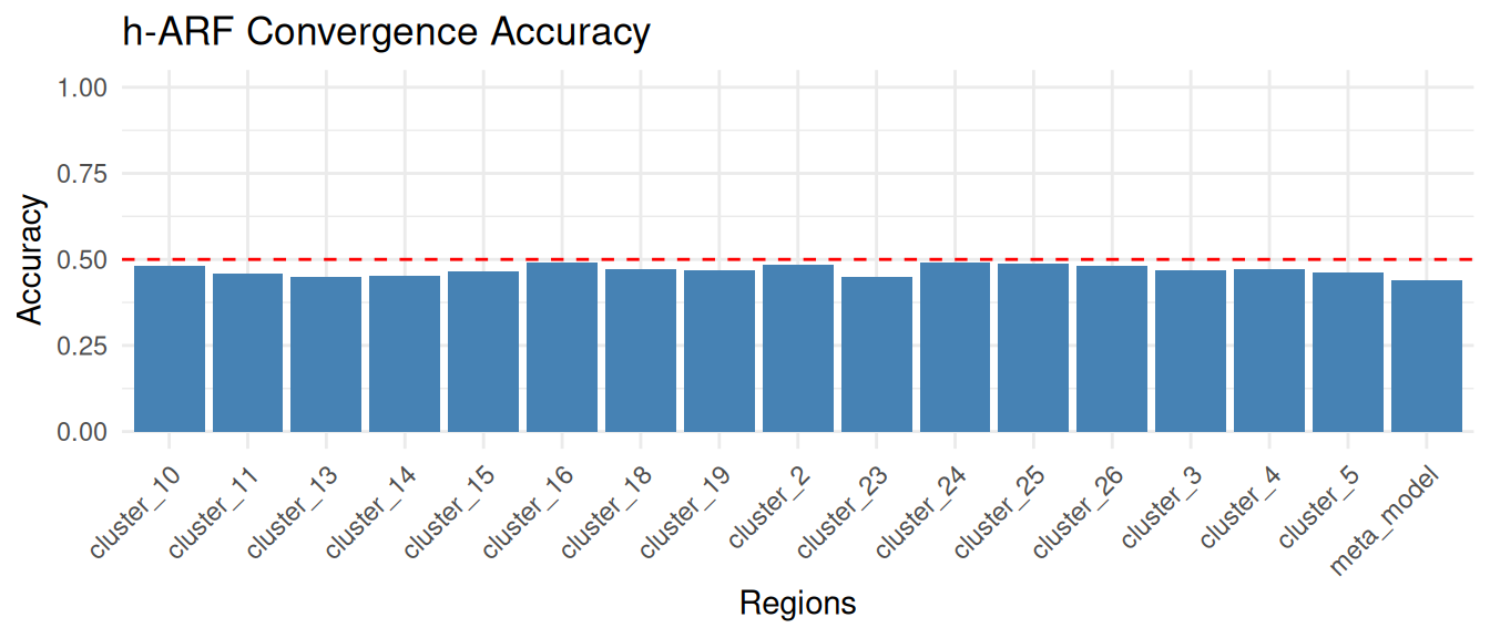

Generating synthetic data

We use the h_forge function to generate sznthsize single cell data using the trained {h}-ARF model. Here, we generate the same number of synthetic samples as in the original dataset, and without any evidence, i.e. without any prio information regarding the the single cell classes (evidence = NULL). As we will see later, the evidence argument can be used to generate synthetic data conditionally on a specific cell types. The generated synthetic data are stored in the synth_single_cell object.

set.seed(32)
synth_single_cell <- h_forge(
  harf_obj = harf_model,
  n_synth = nrow(single_cell), 
  evidence = NULL,
  parallel = FALSE,
  verbose = FALSE
  )

Comparaison of correlation matrices

We visually compare the correlation matrices of the original data and the synthetic data. To enhance interpretability, we rearrange the features according to their region assignments obtained from the {h}-ARF model. The correlation plots exhibit similar patterns across the three datasets, indicating that the {h}-ARF model effectively preserve the origin feature correlation structure.

# Re-arrange data by grouping gene by clusters
cluster_feature <- copy(harf_model$cluster)
setorder(cluster_feature, cluster)
orig_clustered <- single_cell[ , c("cell_type", cluster_feature$feature)]
synth_clustered <- as.data.frame(synth_single_cell)[ , c("cell_type", cluster_feature$feature)]
plot_corr <- function(dt, title) {
  corr_matrix <- cor(dt[ , 2:21], method = "spearman")
  corrplot(corr_matrix,
           method = "circle",
           tl.col = "black",
           tl.pos = "n",
           title = title,
           mar = c(0, 0, 1, 0))
}

Show original and synthetic data in 2D using t-SNE

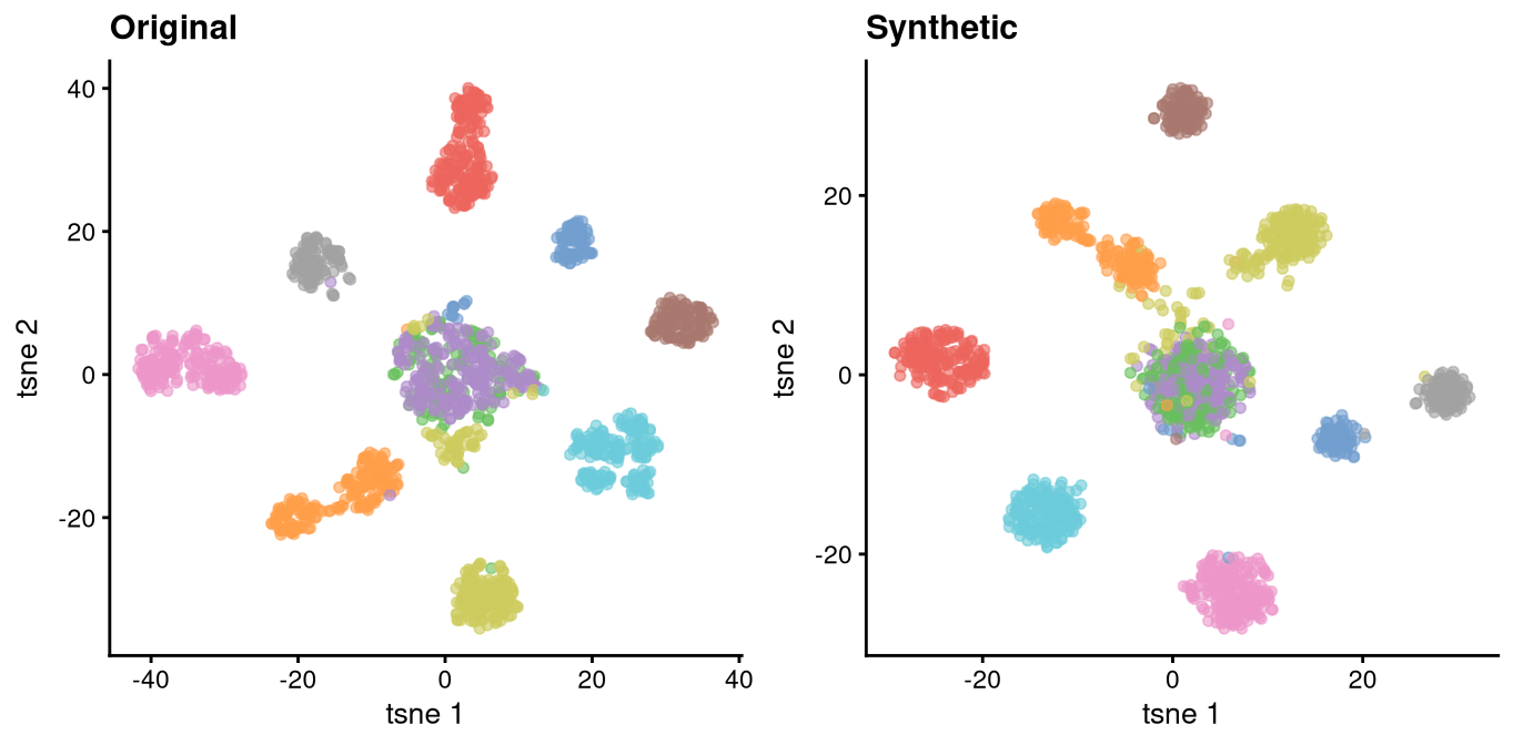
We use t-SNE to visualize cells in a two-dimensional space. Original cell clusters are preserved in the synthetic data, indicating that the {h}-ARF model effectively captures the underlying cluster structure of the original data.

tsne_it <- function (sc_data, perp = 30, title = "") {
  # Create SingleCellExperiment object
  sce <- SingleCellExperiment::SingleCellExperiment(
    assays = list(counts = t(as.matrix(sc_data[ , - which(colnames(sc_data)  == "cell_type")])))
  )
  SingleCellExperiment::logcounts(sce) <- SingleCellExperiment::counts(sce) # Log-normalization
  sce$cell_type <- sc_data$cell_type
  pc_sce <- rpca(t(SingleCellExperiment::counts(sce)))
  # tSNE with rotated pcs
  ts_sce <- Rtsne::Rtsne(
    pc_sce$x %*% pc_sce$rotation,
    perplexity = perp,
    verb = FALSE,
    pca = FALSE,
    check_duplicates = FALSE
  )
  SingleCellExperiment::reducedDim(sce, "tsne") = ts_sce$Y
  sce_plot <- scater::plotReducedDim(sce, "tsne", colour_by = "cell_type") + 
  ggplot2::ggtitle(title) +
  ggplot2::theme(legend.position = "bottom")
  return(sce_plot)
}  
orig_plot <- tsne_it(single_cell,
                     perp = 30,
                     title = "Original")
synth_plot <- tsne_it(as.data.frame(synth_single_cell),
                      perp = 30,
                      title = "Synthetic")
legend <- cowplot::get_legend(
  orig_plot + theme(legend.position = "bottom")
)
orig_plot <- orig_plot + theme(legend.position = "none")
synth_plot <- synth_plot + theme(legend.position = "none")
all_plots <- cowplot::plot_grid(orig_plot,
                                synth_plot,
                                ncol = 2)
par(mfrow = c(1,2))
plot_corr(orig_clustered, "Original")
plot_corr(synth_clustered, "Synthetic")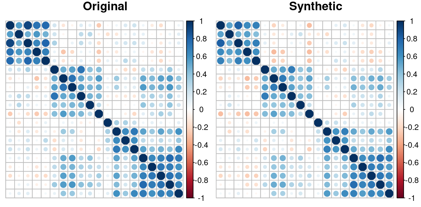

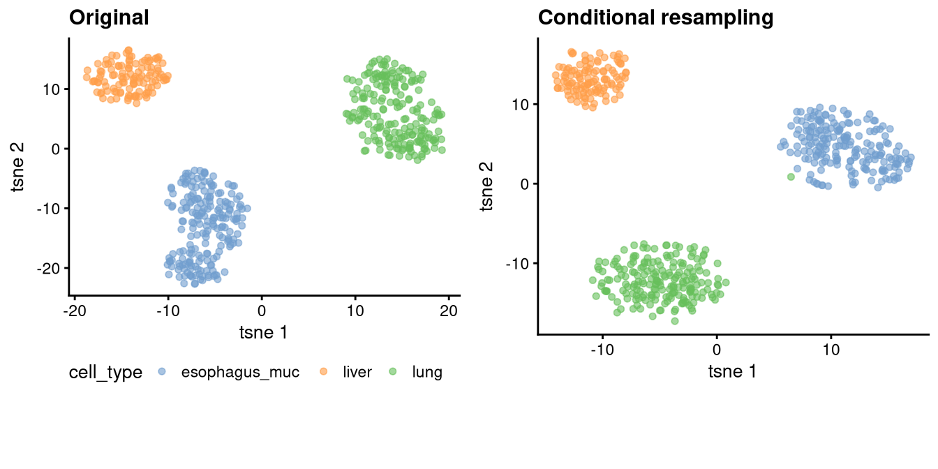
par(mfrow = c(1, 1))
print(all_plots)

Conditional resampling

The evidence parameter is required for conditional resampling. We generate synthetic samples for each cell typ separately. The generated samples are then combined to form the final synthetic dataset. For these example, we synthesize lung, liver and esophagus mucosa cell types. Both the correlation structure and the cluster structure are well preserved in the conditionally generated synthetic data.

sub_cell_type <- c("lung", "liver", "esophagus_muc")
single_cell_list <- lapply(sub_cell_type, function (ct) {
  ct_synth <- h_forge(
        harf_obj = harf_model,
        n_synth = sum(single_cell$cell_type == ct),
        evidence = data.frame(cell_type = ct),
        verbose = FALSE,
        parallel = FALSE
      )
  return(ct_synth)
})
cond_synth_single_cell <- do.call(rbind, single_cell_list)
cond_synth_clustered <- as.data.frame(cond_synth_single_cell)[ , c("cell_type", cluster_feature$feature)]
cond_synth_plot <- tsne_it(as.data.frame(cond_synth_single_cell),
                           perp = 30,
                           title = "Conditional resampling")
sub_legend <- cowplot::get_legend(
  cond_synth_plot + theme(legend.position = "none")
)
cond_synth_plot <- cond_synth_plot + theme(legend.position = "none")
sub_single_cell <- orig_clustered[orig_clustered$cell_type %in% sub_cell_type , ]
sub_orig_plot <- tsne_it(sub_single_cell,
                     perp = 30,
                     title = "Original")
legend <- cowplot::get_legend(
  orig_plot + theme(legend.position = "bottom")
)
sub_all_plots <- cowplot::plot_grid(sub_orig_plot,
                                cond_synth_plot,
                                ncol = 2)
par(mfrow = c(1,2))
plot_corr(sub_single_cell, "Original")
plot_corr(cond_synth_clustered, "Synthetic")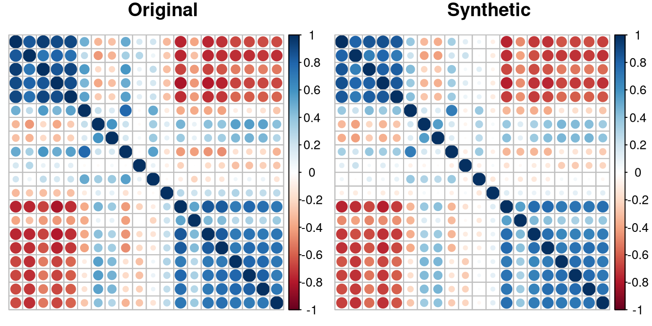

par(mfrow = c(1, 1))
plot_grid(sub_all_plots, sub_legend, ncol = 1, rel_heights = c(1, 0.2))

par(mfrow = c(1, 1))

Again, both the correlation structure and the cluster structure are well preserved in the conditionally generated synthetic data.

Supervised data generating process

The goal is to generate synthetic gene expression data that can be used to evaluate the performance of a prediction model in the absence of original testing datasets, in a situation in which researchers may not have enough samples for eventual internal validation such as corss-validation. As supervised downstream analysis example, we consider the Cancer Genome Atlas Kidney Chromophobe Collection (TCGA-KICH) gene expression predictors, with artificial tumor stage as binary response variable, since the provided original tumor stages were difficult to predict. The dataset contains $66$ samples and the top $140$ gene expression with the highest empirical variances. We include age and gender as additional clinical variables. We scale gene expressions and age. To create the response variable, we fix age and the first $10$ gene expression variables to drive an effect. We set the effect of age to $0.5$ , and draw the effects of gene expressions uniformly from interval $[-1, 1]$ . Subsequently, we train a {h}-ARF model using the h_arf function on the training data, where the gene expression measurements are provided as the omx_data argument, and the binary outcome variable and addition variables including age and gender ( $27$ males and $39$ females) are passed as the cli_lab_data argument. We also specify the target variable using the parameter target. We set the maximal chunk size to $10$ , to specify the maximal number of features allowed in an isolated region. After training the {h}-ARF model, we use the h_forge function to generate synthetic training dataset. We then train a prediction model, on the original and the synthetic training data and evaluate their performances a common testing data. We report the area Receiver Operating Characteristic (ROC) curve (AUC) as performance metric. We expect that the prediction model trained on the synthetic data will have a similar performance to the one trained on the original data, indicating that the {h}-ARF model effectively captures the underlying structure of the original data and can be used to generate realistic synthetic datasets for prediction tasks.

We set up the required libraries.

library(data.table)
library(pROC) # If not installed, use install.packages("pROC") to install it.
library(caret) # If not installed, use install.packages("caret") to install it.
library(ranger) # If not installed, use install.packages("ranger") to install it.
seed <- 123

We load the kich dataset and create training and testing indices.

data("kich")
set.seed(seed)
train_idx <- caret::createDataPartition(
  kich$tumor_stage,
  p = 0.7,
  list = FALSE
)
train_idx <- train_idx[ , "Resample1"]

We use the ranger package to train a random forest model on the original training data and evaluate its performance on the testing data.

Prediction model trained on the original data

set.seed(seed)
rf_model <- ranger(tumor_stage ~ .,
                   data = kich[train_idx, ],
                   num.trees = 500,
                   probability = FALSE)
# Estimate AUC on the test set
test_pred <- predict(rf_model, data = kich[-train_idx, ])$predictions
test_labels <- kich$tumor_stage[-train_idx]
auc_original <- roc(test_labels, as.numeric(test_pred))$auc
print(paste("AUC:", auc_original))
#> [1] "AUC: 0.875"

Supervised adversarial game

We train a {h}-ARF model using the h_arf function on the training data, where the gene expression measurements are provided as the omx_data argument, and the binary outcome variable and addition variables including age and gender are passed as the cli_lab_data argument.

set.seed(seed)
kich_harf <- h_arf(
  omx_data = kich[train_idx , !(colnames(kich) %in% c("tumor_stage",
                                                      "age", "gender"))],
                   cli_lab_data = kich[train_idx, c("tumor_stage", "age", "gender")],
                   chunk_size = 10,
                   target = "tumor_stage",
                   verbose = TRUE
  )
#> Iteration: 0, Accuracy: 43.01%
#> Iteration: 0, Accuracy: 48.39%
#> Iteration: 0, Accuracy: 48.39%
#> Iteration: 0, Accuracy: 35.56%
#> Iteration: 0, Accuracy: 41.49%
#> Iteration: 0, Accuracy: 51.65%
#> Iteration: 1, Accuracy: 39.13%
#> Iteration: 0, Accuracy: 58.51%
#> Iteration: 1, Accuracy: 38.71%
#> Iteration: 0, Accuracy: 56.38%
#> Iteration: 1, Accuracy: 36.56%
#> Iteration: 0, Accuracy: 55.91%
#> Iteration: 1, Accuracy: 44.68%
#> Iteration: 0, Accuracy: 61.7%
#> Iteration: 1, Accuracy: 32.98%
#> Iteration: 0, Accuracy: 56.99%
#> Iteration: 1, Accuracy: 42.55%
#> Iteration: 0, Accuracy: 54.35%
#> Iteration: 1, Accuracy: 40.86%
#> Iteration: 0, Accuracy: 55.91%
#> Iteration: 1, Accuracy: 35.48%
#> Iteration: 0, Accuracy: 51.06%
#> Iteration: 1, Accuracy: 44.57%
#> Iteration: 0, Accuracy: 54.95%
#> Iteration: 1, Accuracy: 38.3%
#> Iteration: 0, Accuracy: 51.61%
#> Iteration: 1, Accuracy: 41.94%
#> Iteration: 0, Accuracy: 56.38%
#> Iteration: 1, Accuracy: 34.78%
#> Iteration: 0, Accuracy: 47.87%
#> Iteration: 0, Accuracy: 55.32%
#> Iteration: 1, Accuracy: 39.36%
#> Iteration: 0, Accuracy: 57.45%
#> Iteration: 1, Accuracy: 48.94%
#> Iteration: 0, Accuracy: 56.52%
#> Iteration: 1, Accuracy: 43.01%

Generating synthetic data

We now use the h_forge function to generate synthetic training dataset.

# Synthetic data
set.seed(seed)
synth_kich <- h_forge(
  harf_obj = kich_harf,
  n_synth = length(train_idx),
  evidence = NULL,
  parallel = FALSE
)
synth_kich <- as.data.frame(synth_kich)

Prediction model trained on the synthetic data

We train a prediction model on the synthetic training data and evaluate its performance on the testing data, the same testing data used to evaluate the model trained on the original data.

set.seed(seed)
rf_model_synth <- ranger(tumor_stage ~ .,
                          data = synth_kich,
                          num.trees = 500,
                          probability = FALSE)
# Estimate AUC on the test set
test_pred_synth <- predict(rf_model_synth, data = kich[-train_idx, ])$predictions
auc_synth <- roc(test_labels, as.numeric(test_pred_synth))$auc
auc_comparison <- data.frame(
  Model = c("Original", "Synthetic"),
  AUC = c(auc_original, auc_synth)
)
print(auc_comparison)
#>       Model   AUC
#> 1  Original 0.875
#> 2 Synthetic 0.875

As expected, the prediction model trained on the synthetic data has a similar performance to the one trained on the original data, indicating that the synthetic datasets can be used for prediction tasks. Our illustration simulated a single run, but in practice, users may want to repeat the process multiple times to assess the variability of the results. As in the unsupervised case, users may also want to tune the chunk size parameter in the adversarial game to achieve a predefined level of performance.

Conclusion

We introduced the R package harf to synthesize high-dimensional data. The package extends the adversarial random forest framework to effectively handle high-dimensional omics data and supports both unconditional and conditional data generation. We have illustrated the usage of the package in both unsupervised and supervised downstream analysis contexts. In the unsupervised context, we demonstrated that the {h}-ARF model can effectively capture the underlying structure of the original data, including the correlation structure between features and the cluster structure of cells. In the supervised context, we showed that synthetic datasets generated by the {h}-ARF model can be used to train prediction models that achieve similar performance to those trained on original data. Therefore, offering a powerful tool for generating realistic synthetic datasets to improve prediction performance in case of lack of training datasets.

References

The Cancer Genome Atlas Pan-Cancer analysis project. Nature Genetics, 45, 1113–1120 (2013). Link here.
The Genotype-Tissue Expression (GTEx) project. Nature Genetics, 47, 1231–1237. (2015). Link here.
Genetic effects on gene expression across human tissues. Nature, 550, 204–213. (2017). Link here.
Q. Wang, J Armenia, C. Zhang, A.V. Penson, E. Reznik, L. Zhang, T. Minet, A. Ochoa, B.E. Gross, C. A. Iacobuzio-Donahue, D. Betel, B.S. Taylor, J. Gao, N. Schultz. Unifying cancer and normal RNA sequencing data from different sources. Scientific Data 5:180061, 2018. Link here.
Fouodo, C. J. K., et al. (2026). High-dimensional adversarial random forests. Submission. Link don’t click.
Watson, D. S., Blesch, K., Kapar, J. & Wright, M. N. (2023). Adversarial random forests for density estimation and generative modeling. In Proceedings of the 26th International Conference on Artificial Intelligence and Statistics. Link here.

Cesaire Fouodo

2026-06-11

Introduction

Unsupervised data generating process

High-dimensional adversarial game

Inspect accuracy of the {h}-ARF model

Generating synthetic data

Comparaison of correlation matrices

Show original and synthetic data in 2D using t-SNE

Conditional resampling

Supervised data generating process

Prediction model trained on the original data

Supervised adversarial game

Generating synthetic data

Prediction model trained on the synthetic data

Conclusion

References